Ensembl Genomic Reference in Bioconductor
TL;DR I gave a talk Genomics in R about querying genomic annotations and references in R/Bioconductor. In this post, we re-visit all the operations in my talk using Ensembl references instead of UCSC/NCBI ones.
This post is part of the “Genomic Data Processing in Bioconductor” series. In that post, I mentioned several topics critical for genomic data analysis in Bioconductor:
- Annotation and genome reference (OrgDb, TxDb, OrganismDb, BSgenome)
- Experiment data storage (ExpressionSets)
- Operations on genome (GenomicRanges)
- Genomic data visualization (Gviz, ggbio)
Few days ago in a local R community meetup, I gave a talk Genomics in R covering the “Annotation and genome reference” part and a quick glance through “Operations on genome”, which should be sufficient for daily usage such as searching annotations in the subset of some genomic ranges. You can find the slides, the meetup screencast (in Chinese) and the accompanied source code online. I don’t think a write-up is needed for the talk. But if anyone is interested, feel free to drop your reply below. :)
Fundamental Bioconductor packages
Some Bioconductor packages are the building blocks for genomic data analysis. I put a table here containing all the classes covered in rest of the post. If you are not familiar with these classes and their methods, go through the talk slides first, or at least follow the annotation workflow on Bioconductor.
| R Class | Description |
|---|---|
OrgDb |
Gene-based information for Homo sapiens; useful for mapping between gene IDs, Names, Symbols, GO and KEGG identifiers, etc. |
TxDb |
Transcriptome ranges for the known gene track of Homo sapiens, e.g., introns, exons, UTR regions. |
OrganismDb |
Collection of multiple annotations for a common organism and genome build. |
BSgenome |
Full genome sequence for Homo sapiens. |
AnnotationHub |
Provides a convenient interface to annotations from many different sources; objects are returned as fully parsed Bioconductor data objects or as the name of a file on disk. |
Ensembl genome browser and its ecosystem
In Bioconductor, most annotations are built against NCBI and UCSC naming systems, which are also used in my talk. However, there is another naming system maintained by Ensembl, whose IDs are very recognizable with suffix “ENSG” and “ENST” for gene and transcript respectively.
I particularly enjoy the Ensembl genome browser. The information is well organized and structured. For example, take a look at the description page of gene MAPK1,
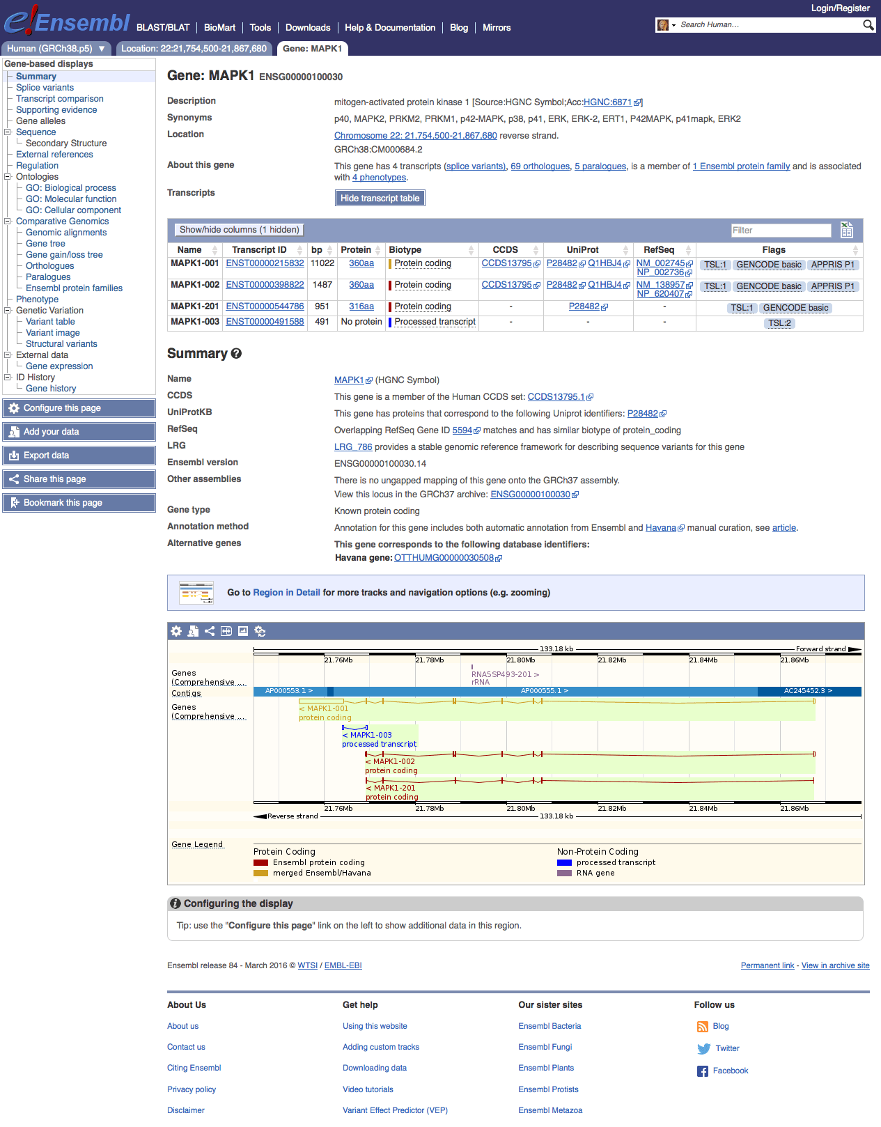
Gene information page of MAP1 on Ensembl Genome Browser release 84 (link)
The gene tree tab shows its homologs and paralogs. The variant table tab shows various kinds of SNPs within MAPK1’s transcript region. SNPs are annotated with their sources, different levels of supporting evidence, and SIFT/PolyPhen prediction on protein function change. Finally, there is a external references tab which links the Ensembl IDs with NCBI CCDS and NCBI RefSeq IDs. There are many ways to explore different aspects of this gene, and it seems everything at multiple biological levels is simply connected.
I always think of the Ensembl ecosystem as a decent learning portal, so it is a pity if one cannot easily use its information in R/Bioconductor. After a quick research, I found using Ensembl annotations are quite straightforward even though the required files does not ship with Bioconductor. Also, there were some topics I failed to mention in the talk, such as AnnotationHub and genomic coordinate system conversion (e.g., from hg19 to hg38). I am going to cover these topics in the talk.
OrgDb
The same OrgDb object for human (org.Hs.eg.db) can be used. It relates different gene IDs, including Entrez and Ensembl gene ID. From its metadata, human’s OrgDb gets updated frequently. Most of its data source were fetched during this March. So one should be able to use it for both hg19 and hg38 human reference.
library(org.Hs.eg.db)
human <- org.Hs.eg.db

mapk_gene_family_info <- select(
    human,
    keys = c("MAPK1", "MAPK3", "MAPK6"),
    keytype = "SYMBOL",
    columns = c("ENTREZID", "ENSEMBL", "GENENAME")
)
mapk_gene_family_info
| SYMBOL | ENTREZID | ENSEMBL | GENENAME |
|---|---|---|---|
| MAPK1 | 5594 | ENSG00000100030 | mitogen-activated protein kinase 1 |
| MAPK3 | 5595 | ENSG00000102882 | mitogen-activated protein kinase 3 |
| MAPK6 | 5597 | ENSG00000069956 | mitogen-activated protein kinase 6 |
Here comes a small pitfall for Ensembl annotation. We cannot sufficiently map Ensembl’s gene ID to its transcript ID,
select(
    human,
    keys = mapk_gene_family_info$ENSEMBL[[1]],
    keytype = "ENSEMBL",
    columns = c("ENSEMBLTRANS")
)
# 'select()' returned 1:1 mapping between keys and columns
#           ENSEMBL ENSEMBLTRANS
# 1 ENSG00000100030         <NA>
We got no Ensembl transcript ID for MAPK1, which is impossible. Therefore, to find the real Ensembl transcript IDs, we need to find other references.
TxDb
There is no pre-built Ensembl TxDb object available on Bioconductor. But with the help of ensembldb, we can easily build the TxDb ourselves.
Following the instructions in ensembldb’s vignette file, we can build the TxDb object from the Ensembl latest release, which is release 84 (Mar, 2016) at the time of writing. Ensembl releases all human transcript records as GTF file, which can be found here ftp://ftp.ensembl.org/pub/release-84/gtf/homo_sapiens/Homo_sapiens.GRCh38.84.gtf.gz.
After processing GTF file via ensDbFromGtf(), the generated data for creating the TxDb object will be stored in a SQLite3 database file Homo_sapiens.GRCh38.84.sqlite at the R working directory. Building TxDB is just one command away, EnsDb(). Putting two commands together, the script for building Ensembl TxDb is listed below. To prevent from rebuilding the TxDb every time the script is executed, we first check if the sqlite file exists,
# xxx_DB in the vignette is just a string to the SQLite db file path
ens84_txdb_pth <- './Homo_sapiens.GRCh38.84.sqlite'
if (!file.exists(ens84_human_txdb_pth)) {
    ens84_txdb_pth <- ensDbFromGtf(gtf="Homo_sapiens.GRCh38.84.gtf.gz")
}
txdb_ens84 <- EnsDb(ens84txdb_pth)
txdb_ens84  # Preview the metadata
The filtering syntax for finding desired genes or transcripts is different to the built-in TxDb object,
transcripts(
    txdb_ens84,
    filter=GeneidFilter(mapk_gene_family_info$ENSEMBL[[1]])
)
# GRanges object with 4 ranges and 5 metadata columns:
#                   seqnames               ranges strand |           tx_id           tx_biotype
#                      <Rle>            <IRanges>  <Rle> |     <character>          <character>
#   ENST00000215832       22 [21754500, 21867629]      - | ENST00000215832       protein_coding
#   ENST00000491588       22 [21763984, 21769428]      - | ENST00000491588 processed_transcript
#   ENST00000398822       22 [21769040, 21867680]      - | ENST00000398822       protein_coding
#   ENST00000544786       22 [21769204, 21867440]      - | ENST00000544786       protein_coding
#                   tx_cds_seq_start tx_cds_seq_end         gene_id
#                          <numeric>      <numeric>     <character>
#   ENST00000215832         21769204       21867440 ENSG00000100030
#   ENST00000491588             <NA>           <NA> ENSG00000100030
#   ENST00000398822         21769204       21867440 ENSG00000100030
#   ENST00000544786         21769204       21867440 ENSG00000100030
#   -------
#   seqinfo: 1 sequence from GRCh38 genome
So filtering is done by passing special filter functions to filter=. Likewise, there are TxidFilter, TxbiotypeFilter, and GRangesFilter for filtering on the respective columns.
tx_gr <- transcripts(
    txdb_ens84,
    filter=TxidFilter("ENST00000215832")
)
tr_gr
# GRanges object with 1 range and 5 metadata columns:
#                   seqnames               ranges strand |           tx_id     tx_biotype tx_cds_seq_start tx_cds_seq_end         gene_id
#                      <Rle>            <IRanges>  <Rle> |     <character>    <character>        <numeric>      <numeric>     <character>
#   ENST00000215832       22 [21754500, 21867629]      - | ENST00000215832 protein_coding         21769204       21867440 ENSG00000100030
#   -------
#   seqinfo: 1 sequence from GRCh38 genome
Check the result with the online Ensembl genome browser. Note that Ensembl release 84 use hg38.
BSgenome and AnnotationHub
We can load the sequence from BSgenome.Hsapiens.UCSC.hg38, however, we can obtain the genome (chromosome) sequence of Ensembl using AnnotationHub. References of non-model organisms can be found on AnnotationHub, many of which are extracted from Ensembl. But they can be downloaded as Bioconductor objects directly so it should be easier to use.
First we create a AnnotationHub instance, it cached the metadata all available annotations locally for us to query.
ah <- AnnotationHub()
query(ah, c("Homo sapiens", "release-84"))
# AnnotationHub with 5 records
# # snapshotDate(): 2016-05-12
# # $dataprovider: Ensembl
# # $species: Homo sapiens
# # $rdataclass: TwoBitFile
# # additional mcols(): taxonomyid, genome, description, tags, sourceurl, sourcetype
# # retrieve records with, e.g., 'object[["AH50558"]]'
#
#             title
#   AH50558 | Homo_sapiens.GRCh38.cdna.all.2bit
#   AH50559 | Homo_sapiens.GRCh38.dna.primary_assembly.2bit
#   AH50560 | Homo_sapiens.GRCh38.dna_rm.primary_assembly.2bit
#   AH50561 | Homo_sapiens.GRCh38.dna_sm.primary_assembly.2bit
#   AH50562 | Homo_sapiens.GRCh38.ncrna.2bit
From the search results, human hg38 genome sequences are available as TwoBit format. But having multiple results is confusing at first. After checking the Ensembl’s gnome DNA assembly readme, what we should use here is the full DNA assembly without any masking (or you can decide it based on your application).
# There are a plenty of query hits. Description of different file suffix:
# GRCh38.dna.*.2bit     genome sequence
# GRCh38.dna_rm.*.2bit  hard-masked genome sequence (masked regions are replaced with N's)
# GRCh38.dna_sm.*.2bit  soft-masked genome sequence (.............. are lower cased)
ens84_human_dna <- ah[["AH50559"]]
Then we can use it to obtain the DNA sequence of desired genomic range (in GRagnes).
getSeq(ens84_human_dna, tx_gr)

#   A DNAStringSet instance of length 1
#      width seq                              names
# [1] 113130 TTTATAGAGAAAA...CTCGGACCGATTGCCT ENST00000215832
biomaRt
BioMart are a collections of database that can be accessed by the same API, including Ensembl, Uniprot and HapMap. biomaRt provides an R interface to these database resources. We will use BioMart for ID conversion between Ensembl and RefSeq. Its vignette contains solutions to common scenarios so should be a good starting point to get familiar with it.
You could first explore which Marts are currently available by listMarts(),
library(biomaRt)
listMarts()
#                biomart               version
# 1 ENSEMBL_MART_ENSEMBL      Ensembl Genes 84
# 2     ENSEMBL_MART_SNP  Ensembl Variation 84
# 3 ENSEMBL_MART_FUNCGEN Ensembl Regulation 84
# 4    ENSEMBL_MART_VEGA               Vega 64
Here we will use Ensembl’s biomart. Each mart contains multiple datasets, usually separated by different organisms. In our case, human’s dataset is hsapiens_gene_ensembl. For other organisms, you can find their dataset by listDatasets(ensembl).
ensembl <- useMart("ensembl")
ensembl <- useDataset("hsapiens_gene_ensembl", mart=ensembl)
# or equivalently
ensembl <- useMart("ensembl", dataset="hsapiens_gene_ensembl")
Compatibility with AnnotationDb’s interface
The way to query the ensembl Mart object is slightly different to how we query a AnnotationDb object. The major difference is the terminology. Luckily, Mart object provides a compatibility layer so we can still call functions such as select(db, ...), keytypes(db), keys(db) and columns(db), which we frequently do1 when using NCBI/UCSC references.
A Mart can have hundreds of keys and columns. So we select a part of them out by grep(),
grep("^refseq", keytypes(ensembl), value = TRUE)
# [1] "refseq_mrna" "refseq_mrna_predicted" ...
grep("^ensembl", keytypes(ensembl), value = TRUE)
# [1] "ensembl_exon_id" "ensembl_gene_id" ...
grep("hsapiens_paralog_", columns(ensembl), value=TRUE)
# [1] "hsapiens_paralog_associated_gene_name"
# [2] "hsapiens_paralog_canonical_transcript_protein"
# [3] "hsapiens_paralog_chrom_end"
# ...
We start by finding the MAPK1’s RefSeq transcript IDs and their corresponding Ensembl transcript IDs, which is something we cannot do by our locally built Ensembl TxDb nor the human OrgDb.
select(
    ensembl,
    keys = c("MAPK1"),
    keytype = "hgnc_symbol",
    columns =  c(
        "refseq_mrna", "ensembl_transcript_id",
        "hgnc_symbol", "entrezgene",
        "chromosome_name",
        "transcript_start", "transcript_end", "strand"
    )
)
#   refseq_mrna ensembl_transcript_id hgnc_symbol entrezgene
# 1   NM_002745       ENST00000215832       MAPK1       5594
# 2                   ENST00000491588       MAPK1       5594
# 3   NM_138957       ENST00000398822       MAPK1       5594
# 4                   ENST00000544786       MAPK1       5594
#   chromosome_name transcript_start transcript_end strand
# 1              22         21754500       21867629     -1
# 2              22         21763984       21769428     -1
# 3              22         21769040       21867680     -1
# 4              22         21769204       21867440     -1
So some of the MAPK1 Ensembl transcripts does not have RefSeq identifiers. This is common to see since RefSeq is more conservative about including new transcripts. Anyway, we can now translate our analysis result between a wider range of naming systems.
Moreover, what’s awesome about BioMart is that almost all the information on the Ensembl genome browser can be retreived by BioMart. For example, getting the paralog and the mouse homolog of MAPK1,
# Get paralog of MAPK1
select(
    ensembl,
    keys = c("ENSG00000100030"),
    keytype = "ensembl_gene_id",
    columns = c(
        "hsapiens_paralog_associated_gene_name",
        "hsapiens_paralog_orthology_type",
        "hsapiens_paralog_ensembl_peptide"
    )
)
#   hsapiens_paralog_associated_gene_name hsapiens_paralog_orthology_type hsapiens_paralog_ensembl_peptide
# 1                                 MAPK3          within_species_paralog                  ENSP00000263025
# 2                                 MAPK6          within_species_paralog                  ENSP00000261845
# 3                                 MAPK4          within_species_paralog                  ENSP00000383234
# 4                                   NLK          within_species_paralog                  ENSP00000384625
# 5                                 MAPK7          within_species_paralog                  ENSP00000311005

# Get homolog of MAPK1 in mouse
select(
    ensembl,
    keys = c("ENSG00000100030"),
    keytype = "ensembl_gene_id",
    columns = c(
        "mmusculus_homolog_associated_gene_name",
        "mmusculus_homolog_orthology_type",
        "mmusculus_homolog_ensembl_peptide"
    )
)
#   mmusculus_homolog_associated_gene_name mmusculus_homolog_orthology_type mmusculus_homolog_ensembl_peptide
# 1                                  Mapk1                 ortholog_one2one                ENSMUSP00000065983
biomaRt’s original interface
The select() function we use is not the original biomaRt’s interface. In fact, keys and columns are interpreted as BioMart’s filters and attributes respectively. To find all available filters and attributes,
filters = listFilters(ensembl)
attributes = listAttributes(ensembl)
each of the command return a data.frame that contains each filter’s or attribute’s name and description.
Behind the scene, arguments of select(db, ...) is converted to getBM(mart, ...). For the same example of finding RefSeq and Ensembl transcript IDs, it can be re-written as
getBM(
    attributes = c(
        "refseq_mrna", "ensembl_transcript_id",
        "chromosome_name",
        "transcript_start", "transcript_end", "strand",
        "hgnc_symbol", "entrezgene", "ensembl_gene_id"
    ),
    filters = "hgnc_symbol",
    values = c("MAPK1"),
    mart = ensembl
)
Conversion between genomic coordinate systems
Somethings we need to convert between different verions of the reference. For example, today we’d like to convert a batch of genomic locations of reference hg38 to that of hg19, so we can compare our new research with previous studies. It is a non-trivial task that can be currently handled by the following tools:
Frankly I don’t have experience for such conversion in real study (the converted result still gives the sense of unease), but anyway here I follow the guide on PH525x series. In Bioconductor, we can use UCSC’s Chain file to apply the liftOver() method provided by package rtracklayer. To convert regions from hg38 to hg19, we need the hg38ToHg19.over.chain file, which can be found at ftp://hgdownload.cse.ucsc.edu/goldenPath/hg38/liftOver/.
We still use MAPK1 as an example of conversion. First extract MAPK1’s genomic ranges in hg38 and hg19 respectively,
library(TxDb.Hsapiens.UCSC.hg38.knownGene)
library(TxDb.Hsapiens.UCSC.hg19.knownGene
tx38 <- TxDb.Hsapiens.UCSC.hg38.knownGene
tx19 <- TxDb.Hsapiens.UCSC.hg19.knownGene
MAPK1_hg38 <- genes(tx38, filter=list(gene_id="5594"))
MAPK1_hg19 <- genes(tx19, filter=list(gene_id="5594"))
Then we convert MAPK1_hg38 to use the hg19 coordinate system.
library(rtracklayer)
ch <- import.chain("./hg38ToHg19.over.chain")
MAPK1_hg19_lifted <- liftOver(MAPK1_hg38, ch)

MAPK1_hg19
# GRanges object with 1 range and 1 metadata column:
#        seqnames               ranges strand |     gene_id
#           <Rle>            <IRanges>  <Rle> | <character>
#   5594    chr22 [22113947, 22221970]      - |        5594
#   -------
#   seqinfo: 93 sequences (1 circular) from hg19 genome

MAPK1_hg19_lifted
# GRangesList object of length 1:
# $5594
# GRanges object with 2 ranges and 1 metadata column:
#       seqnames               ranges strand |     gene_id
#          <Rle>            <IRanges>  <Rle> | <character>
#   [1]    chr22 [22113947, 22216652]      - |        5594
#   [2]    chr22 [22216654, 22221970]      - |        5594
#
# -------
# seqinfo: 1 sequence from an unspecified genome; no seqlengths
So the conversion worked as expected, though it created a gap in the range (missing a base at 22216653). I haven’t looked into the results. To ensure the correctness of the conversion, maybe a comparison with CrossMap is needed.
Summary
We skimmed through OrgDb and TxDb again using the Ensembl references, including how to build the TxDb for Ensembl locally and obtain external annotations from AnnotationHub.
BioMart is an abundant resource to query across various types of databases and references, which can be used in conversion between different naming systems.
Finally, we know how to convert between different version of the reference. Though the correctness of the conversion requires further examination (not meaning it is wrong), at least the conversion by liftOver works as expected.
Starting here, you should have no trouble dealing with annotations in R anymore. For the next post, I plan to further explore the way to read sequencing analysis results in R.
-
Note that the
select(mart, ...)compatibility does not apply to all existed filters (keys) and attributes (columns) of the given Mart. ↩