Genomics in R
Esc to overview
← → to navigate

Liang-Bo Wang (亮亮), 2016-05-16
By Liang2 under CC 4.0 BY license
Esc to overview
← → to navigate


Bioconductor provides tools for the analysis and comprehension of high-throughput genomic data.
source("https://bioconductor.org/biocLite.R")biocLite("PKGNAME")
source("https://bioconductor.org/biocLite.R")
biocLite()   # install fundamental packages
biocLite(c(  # packages required for today's demo
    "Homo.sapiens",
    "BSgenome.Hsapiens.UCSC.hg19",
))
install.packages(c("devtools", "stringr", "plyr"))
| Object Type | Example Package Name |
|---|---|
| OrgDb | org.Hs.eg.db |
| TxDb | TxDb.Hsapiens.UCSC.hg19.knownGene |
| BSgenome | BSgenome.Hsapiens.UCSC.hg19 |
| OrganismDb | Homo.sapiens |
| AnnotationHub | AnnotationHub |
Ref: Bioconductor workflow – Annotation Resources.
Bioconductor contains hundreds of these AnnotationData packages.
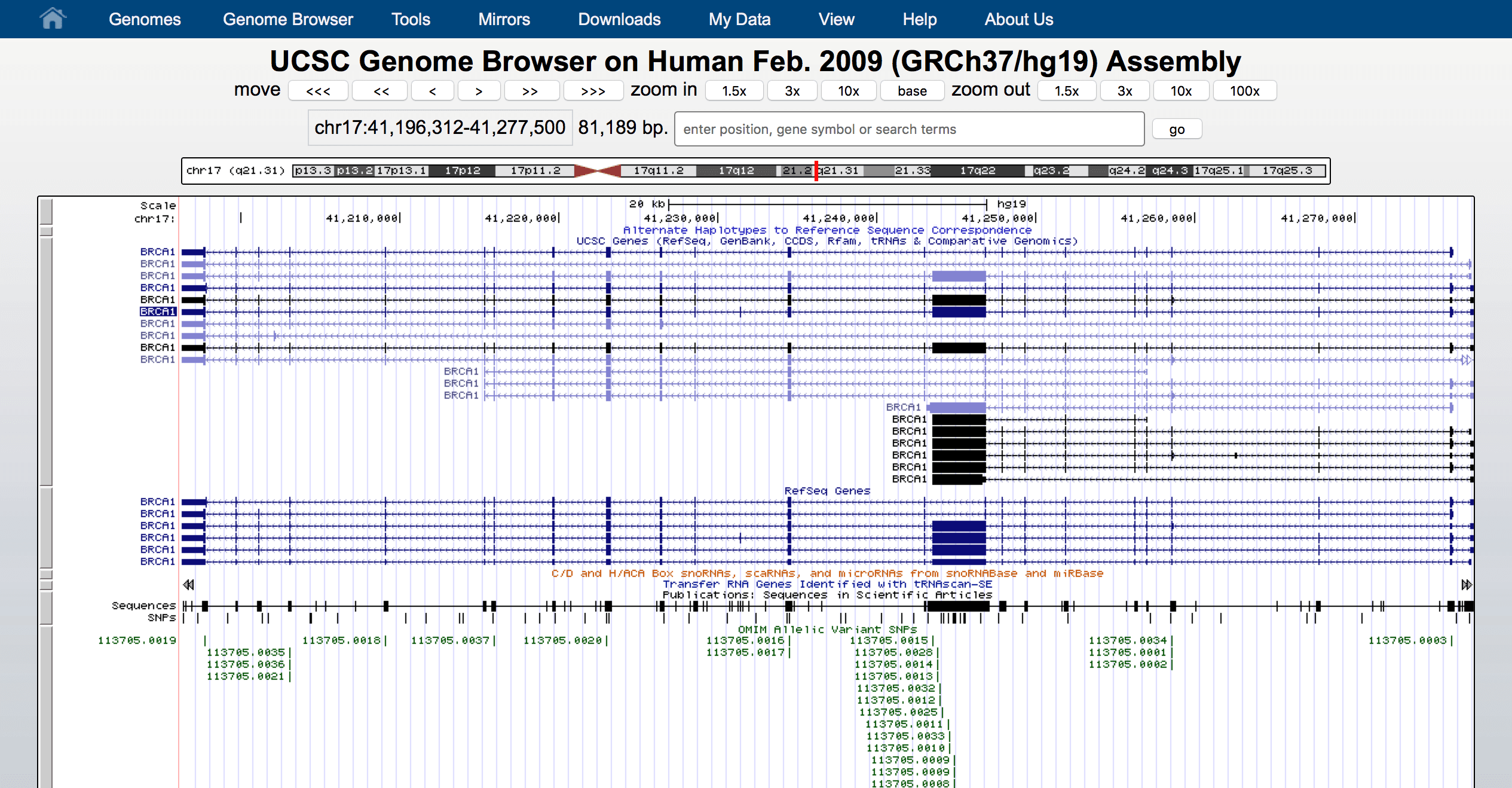
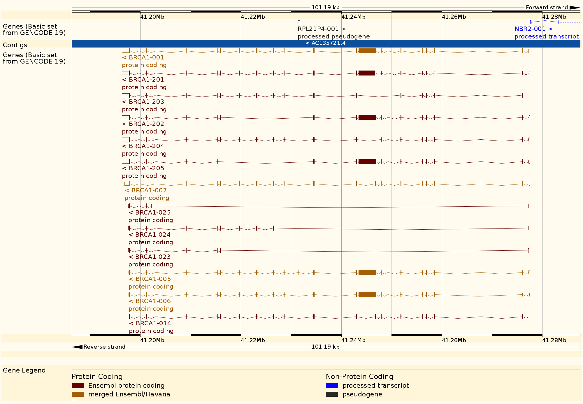
We can use these annotation sources to act as a simple genome browser. Here we use Bioconductor to show gene GAPDH in human genome hg19.
devtools::install_github("genomicsclass/ph525x")
biocLite("Gviz")  # Gviz for plotting genomic data
library(ph525x)  # Provides handy helper functions

modPlot("GAPDH", collapse=FALSE, useGeneSym=FALSE)
Ref: Annotating phenotypes and molecular function from PH525x series
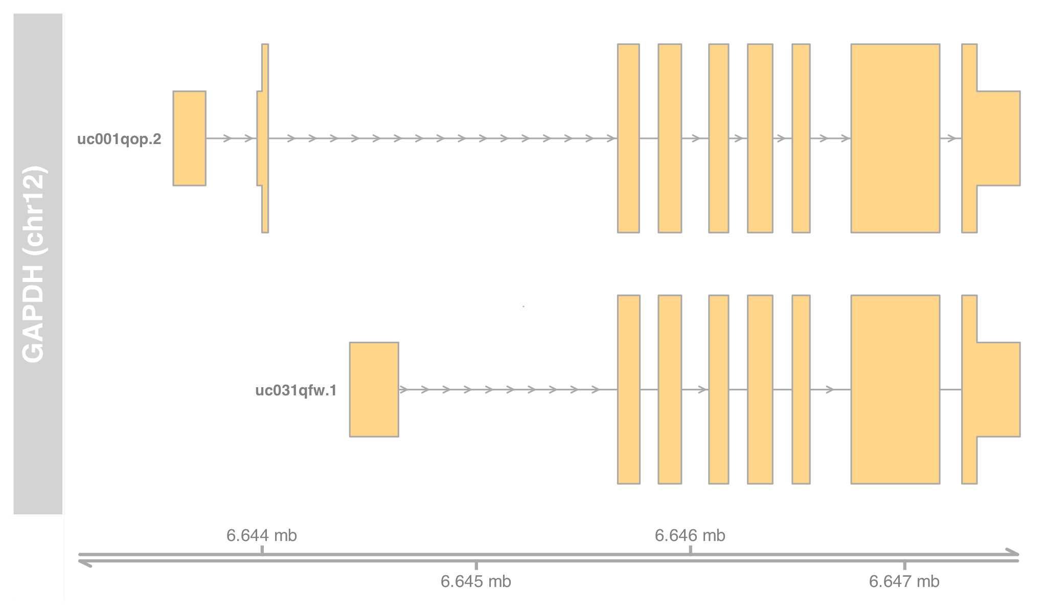
Behind the scene, modPlot(...) did a lot of queries. Let's find out how to extract this information ourselves using the annotation related API.
Plot is made by Gviz. Though we are not able to introduce it today.
columns(), keytypes(), keys()select(), mapIds()
	> human
OrgDb object:
| DBSCHEMAVERSION: 2.1
| Db type: OrgDb
| Supporting package: AnnotationDbi
| DBSCHEMA: HUMAN_DB
| ORGANISM: Homo sapiens
| SPECIES: Human
| EGSOURCEDATE: 2016-Mar14
| EGSOURCENAME: Entrez Gene
| EGSOURCEURL: ftp://ftp.ncbi.nlm.nih.gov/gene/DATA
| CENTRALID: EG
| TAXID: 9606
| GOSOURCENAME: Gene Ontology
| GOSOURCEURL: ftp://ftp.geneontology.org/pub/go/godatabase/archive/latest-lite/
| GOSOURCEDATE: 20160305
| GOEGSOURCEDATE: 2016-Mar14
| GOEGSOURCENAME: Entrez Gene
| GOEGSOURCEURL: ftp://ftp.ncbi.nlm.nih.gov/gene/DATA
| KEGGSOURCENAME: KEGG GENOME
| KEGGSOURCEURL: ftp://ftp.genome.jp/pub/kegg/genomes
| KEGGSOURCEDATE: 2011-Mar15
| GPSOURCENAME: UCSC Genome Bioinformatics (Homo sapiens)
| GPSOURCEURL: ftp://hgdownload.cse.ucsc.edu/goldenPath/hg19
| GPSOURCEDATE: 2010-Mar22
| ENSOURCEDATE: 2016-Mar9
| ENSOURCENAME: Ensembl
| ENSOURCEURL: ftp://ftp.ensembl.org/pub/current_fasta
| UPSOURCENAME: Uniprot
| UPSOURCEURL: http://www.UniProt.org/
| UPSOURCEDATE: Wed Mar 23 15:50:09 2016
Many metadata about each annotation's original source and last update date can be found here.
library(org.Hs.eg.db)
human <- org.Hs.eg.db
columns(human)  # shows all available columns
# "ACCNUM"   "ALIAS"  "ENSEMBL"  "ENSEMBLPROT" "ENSEMBLTRANS"
# "ENTREZID" "ENZYME" "EVIDENCE" "EVIDENCEALL" "GENENAME"
# "GO" "GOALL" "IPI"  "MAP" "OMIM" "ONTOLOGY"  "ONTOLOGYALL" ...
org.Hs.eg.db's "eg" means data come from NCBI Entrez Gene. Info about each column can be found by help("ENSEMBL")
keytypes(orgDb).keys() return values of the given column.
keys(human, "SYMBOL")  # [1] "A1BG" "A2M" "A2MP1" ...

# Passed a pattern to filter the returned symbols
keys(human, keytype="SYMBOL", pattern="MAPK")
# [1] "MAPK14" "MAPK1" "MAPK3" "MAPK4" "MAPK6" "MAPK7" ...
# Accept regex as well
keys(human, keytype="SYMBOL", pattern="^MAPK[[:digit:]]{2}$")
# [1] "MAPK14" "MAPK11" "MAPK10" "MAPK13" "MAPK12" "MAPK15"
select() connects different columns. Say, what are the Entrez Gene IDs and their full name for MAPK gene family?
select(
    human,
    keys = c("MAPK1", "MAPK3", "MAPK6"),
    keytype = "SYMBOL",
    columns = c("ENTREZID", "GENENAME")
)
# select(...) from the last page
# 'select()' returned 1:1 mapping between keys and columns
  SYMBOL ENTREZID                           GENENAME
1  MAPK1     5594 mitogen-activated protein kinase 1
2  MAPK3     5595 mitogen-activated protein kinase 3
3  MAPK6     5597 mitogen-activated protein kinase 6
How does these functions interact with the underlying database?
-- Get SQLite3 database filepath by `dbfile(org.Hs.eg.db)`
sqlite> SELECT symbol, gene_id AS entrez_id, gene_name
   ...> FROM genes JOIN (
   ...>     SELECT * FROM gene_info
   ...>     WHERE symbol IN ("MAPK1", "MAPK3", "MAPK6")
   ...> ) AS symbol_info
   ...> ON genes._id = symbol_info._id;
symbol	entrez_id	gene_name
MAPK1	5594		mitogen-activated protein kinase 1
MAPK3	5595		mitogen-activated protein kinase 3
MAPK6	5597		mitogen-activated protein kinase 6
For example, find all RefSeq IDs for these MAPK-family genes.
select(
    human,
    keys = MAPKS,
    keytype = "SYMBOL",
    columns = c("REFSEQ")
)
# 'select()' returned 1:many ...
   SYMBOL       REFSEQ
1   MAPK1    NM_002745
2   MAPK1    NM_138957
3   MAPK1    NP_002736
4   MAPK1    NP_620407
5   MAPK3 NM_001040056
6   MAPK3 NM_001109891
# ...
Use mapIds(multiVals="list"), which returns a list-like structure grouped by having the same key (here is SYMBOL).
refseq_ids <- mapIds(
    human,
    keys = MAPKS,
    keytype = "SYMBOL",
    column = "REFSEQ",
    multiVals = "list"
)
$MAPK1
[1] "NM_002745" "NM_138957" ...
$MAPK3
[1] "NM_001040056" "NM_001109891"
$MAPK6
[1] "NM_002748" "NP_002739" ...
# ...
refseq_ids$MAPK1  # operate exactly as a list
# [1] "NM_002745" "NM_138957" "NP_002736" "NP_620407"

lapply(  # select only transcript IDs (starting with "NM_")
    refseq_ids,
	function(ids) grep("^NM_", ids, value = TRUE)
)
# $MAPK1
# [1] "NM_002745" "NM_138957"
# $MAPK3
# [1] "NM_001040056" "NM_001109891" "NM_002746" ...
library(TxDb.Hsapiens.UCSC.hg19.knownGene)
txdb <- TxDb.Hsapiens.UCSC.hg19.knownGene
keytypes(txdb)
# [1] "CDSID" "CDSNAME" "EXONID" "EXONNAME" "GENEID"
# [6] "TXID" "TXNAME"
columns(txdb)
#  [1] "CDSCHROM" "CDSEND" "CDSID" "CDSNAME" "CDSSTART"
#  [6] "CDSSTRAND" "EXONCHROM" "EXONEND" "EXONID" "EXONNAME"
# [11] "EXONRANK" "EXONSTART" "EXONSTRAND" "GENEID" "TXCHROM"
# [16] "TXEND" "TXID" "TXNAME" "TXSTART" "TXSTRAND" "TXTYPE"
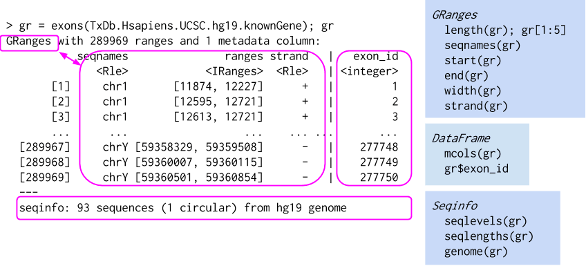
transcripts(txdb) returns all transcript records (in GRanges).
txs <- transcripts(txdb); txs
# GRanges object with 82960 ranges and 2 metadata columns:
#                 seqnames           ranges strand |     tx_id     tx_name
#                    <Rle>        <IRanges>  <Rle> | <integer> <character>
#       [1]           chr1 [ 11874,  14409]      + |         1  uc001aaa.3
#       [2]           chr1 [ 11874,  14409]      + |         2  uc010nxq.1
#       [3]           chr1 [ 11874,  14409]      + |         3  uc010nxr.1
#       [4]           chr1 [ 69091,  70008]      + |         4  uc001aal.1
#       [5]           chr1 [321084, 321115]      + |         5  uc001aaq.2
#       ...            ...              ...    ... .       ...         ...
#   [82956] chrUn_gl000237   [    1,  2686]      - |     82956  uc011mgu.1
#   [82957] chrUn_gl000241   [20433, 36875]      - |     82957  uc011mgv.2
#   [82958] chrUn_gl000243   [11501, 11530]      + |     82958  uc011mgw.1
#   [82959] chrUn_gl000243   [13608, 13637]      + |     82959  uc022brq.1
#   [82960] chrUn_gl000247   [ 5787,  5816]      - |     82960  uc022brr.1
#   -------
#   seqinfo: 93 sequences (1 circular) from hg19 genome
Similar extractor functions exist for genes(), exons(), cds().
genes <- genes(txdb); genes
# GRanges object with 23056 ranges and 1 metadata column:
#         seqnames                 ranges strand |     gene_id
#            <Rle>              <IRanges>  <Rle> | <character>
#       1    chr19 [ 58858172,  58874214]      - |           1
#      10     chr8 [ 18248755,  18258723]      + |          10
#     100    chr20 [ 43248163,  43280376]      - |         100
#    1000    chr18 [ 25530930,  25757445]      - |        1000
#   10000     chr1 [243651535, 244006886]      - |       10000
#     ...      ...                    ...    ... .         ...
#    9991     chr9 [114979995, 115095944]      - |        9991
#    9992    chr21 [ 35736323,  35743440]      + |        9992
#    9993    chr22 [ 19023795,  19109967]      - |        9993
#    9994     chr6 [ 90539619,  90584155]      + |        9994
#    9997    chr22 [ 50961997,  50964905]      - |        9997
#   -------
#   seqinfo: 93 sequences (1 circular) from hg19 genome
Can subset the GRanges object via the row id (gene_id).
genes[c("5594", "5595")]
# GRanges object with 2 ranges and 1 metadata column:
#        seqnames               ranges strand |     gene_id
#           <Rle>            <IRanges>  <Rle> | <character>
#   5594    chr22 [22113947, 22221970]      - |        5594
#   5595    chr16 [30125426, 30134630]      - |        5595
#   -------
#   seqinfo: 93 sequences (1 circular) from hg19 genome
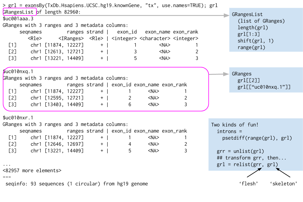
How to find transcripts of a gene? How to know the extrons, UTRs of a transcripts?
transcriptsBy(txdb, by = "gene")exonsBy(txdb, by = "tx", use.names = TRUE)
txby <- transcriptsBy(txdb, by="gene"); txby
# GRangesList object of length 23459:
# $1
# GRanges object with 2 ranges and 2 metadata columns:
#       seqnames               ranges strand |     tx_id     tx_name
#          <Rle>            <IRanges>  <Rle> | <integer> <character>
#   [1]    chr19 [58858172, 58864865]      - |     70455  uc002qsd.4
#   [2]    chr19 [58859832, 58874214]      - |     70456  uc002qsf.2
#
# $10
# GRanges object with 1 range and 2 metadata columns:
#       seqnames               ranges strand | tx_id    tx_name
#   [1]     chr8 [18248755, 18258723]      + | 31944 uc003wyw.1
#
# ...
# <23456 more elements>
# -------
# seqinfo: 93 sequences (1 circular) from hg19 genome
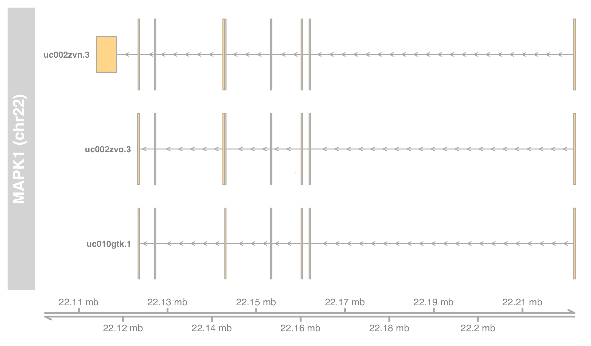
transcriptsBy() returns a GRangesList, whose keys are gene IDs (Entrez). Select MAPK1's transcripts and verify with what we found in OrgDb.
txby[["5594"]]
# GRanges object with 3 ranges and 2 metadata columns:
#       seqnames               ranges strand |     tx_id     tx_name
#          <Rle>            <IRanges>  <Rle> | <integer> <character>
#   [1]    chr22 [22113947, 22221970]      - |     74608  uc002zvn.3
#   [2]    chr22 [22123319, 22221970]      - |     74609  uc002zvo.3
#   [3]    chr22 [22123484, 22221970]      - |     74610  uc010gtk.1
#   -------
#   seqinfo: 93 sequences (1 circular) from hg19 genome
Why we know the gene IDs are Entrez Gene IDs? (try printing txdb itself)
exby <- exonsBy(txdb, by = "tx", use.names = TRUE); exby
# GRangesList object of length 82960:
# $uc001aaa.3
# GRanges object with 3 ranges and 3 metadata columns:
#       seqnames         ranges strand |   exon_id   exon_name exon_rank
#          <Rle>      <IRanges>  <Rle> | <integer> <character> <integer>
#   [1]     chr1 [11874, 12227]      + |         1        <NA>         1
#   [2]     chr1 [12613, 12721]      + |         3        <NA>         2
#   [3]     chr1 [13221, 14409]      + |         5        <NA>         3
#
# $uc010nxq.1
# GRanges object with 3 ranges and 3 metadata columns:
#       seqnames         ranges strand | exon_id exon_name exon_rank
#   [1]     chr1 [11874, 12227]      + |       1      <NA>         1
#   [2]     chr1 [12595, 12721]      + |       2      <NA>         2
#   [3]     chr1 [13403, 14409]      + |       6      <NA>         3
#
# ...
# <82957 more elements>
# -------
# seqinfo: 93 sequences (1 circular) from hg19 genome
exonsBy() returns a GRangesList, whose keys are transcript IDs (UCSC KnownGene). Pick one MAPK1 transcript and verify with modPlot()'s result.
exby[["uc002zvn.3"]]
# GRangesList object of length 1:
# $uc002zvn.3
# GRanges object with 9 ranges and 3 metadata columns:
#       seqnames               ranges strand |   exon_id   exon_name exon_rank
#          <Rle>            <IRanges>  <Rle> | <integer> <character> <integer>
#   [1]    chr22 [22221612, 22221970]      - |    264662        <NA>         1
#   [2]    chr22 [22161953, 22162135]      - |    264661        <NA>         2
#   [3]    chr22 [22160139, 22160328]      - |    264660        <NA>         3
#   ...
#   [7]    chr22 [22127162, 22127271]      - |    264656        <NA>         7
#   [8]    chr22 [22123484, 22123609]      - |    264655        <NA>         8
#   [9]    chr22 [22113947, 22118529]      - |    264653        <NA>         9
#
# -------
# seqinfo: 93 sequences (1 circular) from hg19 genome
Extract the chromosome information by seqinfo(), returning a Seqinfo object. Works on all GRanges objects.
si <- seqinfo(txdb); si
# Seqinfo object with 93 sequences (1 circular) from hg19 genome:
#   seqnames       seqlengths isCircular genome
#   chr1            249250621       <NA>   hg19
#   chr2            243199373       <NA>   hg19
#   chr3            198022430       <NA>   hg19
#   ...                   ...        ...    ...
#   chrUn_gl000247      36422       <NA>   hg19
#   chrUn_gl000248      39786       <NA>   hg19
#   chrUn_gl000249      38502       <NA>   hg19
seqnames(si)  # use its column name as function
# [1] "chr1" "chr2" "chr3" "chr4" "chr5" ...
seqlengths(si)
#      chr1      chr2      chr3      chr4      chr5 ...
# 249250621 243199373 198022430 191154276 180915260 ...
isCircular(si)
# chr1 chr2 chr3 chr4 chr5 ... chrM ...
#   NA   NA   NA   NA   NA ... TRUE ...
For example, Ensembl uses NCBI style naming (1, 2, ...); UCSC prefix all chromosome names with "chr".
seqlevels(txdb)
# [1] "chr1" "chr2" "chr3" "chr4" "chr5" "chr6" ...
seqlevelsStyle(txdb)
# [1] "UCSC"
seqlevelsStyle(txdb) <- "NCBI"  # change the naming style
seqlevels(txdb)
# [1] "1" "2" "3" "4" "5" "6" ...
columns() and select())transcripts() and genes())transcriptsBy() and exonsBy())seqinfo()Homo.sapiens
library(Homo.sapiens)
human <- Homo.sapiens
	> human
OrganismDb Object:
# Includes GODb Object:  GO.db
# With data about:  Gene Ontology
# Includes OrgDb Object:  org.Hs.eg.db
# Gene data about:  Homo sapiens
# Taxonomy Id:  9606
# Includes TxDb Object:  TxDb.Hsapiens.UCSC.hg19.knownGene
# Transcriptome data about:  Homo sapiens
# Based on genome:  hg19
# The OrgDb gene id ENTREZID is mapped to
# the TxDb gene id GENEID .
select(
    human,
    keys = c("MAPK1"), keytype = "SYMBOL",
    columns = c("TXNAME", "TXCHROM", "TXSTRAND")
)
#   SYMBOL     TXNAME TXCHROM TXSTRAND
# 1  MAPK1 uc002zvn.3   chr22        -
# 2  MAPK1 uc002zvo.3   chr22        -
# 3  MAPK1 uc010gtk.1   chr22        -
transcripts(human, columns=c("TXNAME", "SYMBOL"))
# 'select()' returned 1:1 mapping between keys and columns
# GRanges object with 82960 ranges and 2 metadata columns:
#                 seqnames           ranges strand |          TXNAME          SYMBOL
#                    <Rle>        <IRanges>  <Rle> | <CharacterList> <CharacterList>
#       [1]           chr1 [ 11874,  14409]      + |      uc001aaa.3         DDX11L1
#       [2]           chr1 [ 11874,  14409]      + |      uc010nxq.1         DDX11L1
#       [3]           chr1 [ 11874,  14409]      + |      uc010nxr.1         DDX11L1
#       [4]           chr1 [ 69091,  70008]      + |      uc001aal.1           OR4F5
#       [5]           chr1 [321084, 321115]      + |      uc001aaq.2              NA
#       ...            ...              ...    ... .             ...             ...
#   [82956] chrUn_gl000237   [    1,  2686]      - |      uc011mgu.1              NA
#   [82957] chrUn_gl000241   [20433, 36875]      - |      uc011mgv.2              NA
#   [82958] chrUn_gl000243   [11501, 11530]      + |      uc011mgw.1              NA
#   [82959] chrUn_gl000243   [13608, 13637]      + |      uc022brq.1              NA
#   [82960] chrUn_gl000247   [ 5787,  5816]      - |      uc022brr.1              NA
#   -------
#   seqinfo: 93 sequences (1 circular) from hg19 genome
But how can we get the contents columns like TXNAME and SYMBOL?!
Ref: Genomic Ranges For Genome-Scale Data And Annotation, Martin Morgan, 2015.10
Ref: Genomic Ranges For Genome-Scale Data And Annotation, Martin Morgan, 2015.10
?"intra-range-methods")?"inter-range-methods")Ref: Genomic Ranges For Genome-Scale Data And Annotation, Martin Morgan, 2015.10
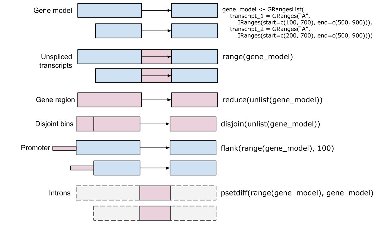
Ref: Genomic Ranges For Genome-Scale Data And Annotation, Martin Morgan, 2015.10
txs <- transcripts(human, columns=c("TXNAME", "SYMBOL"))
mcols(txs)  # act as data.frame
# DataFrame with 82960 rows and 2 columns
#                TXNAME          SYMBOL
#       <CharacterList> <CharacterList>
# 1          uc001aaa.3         DDX11L1
# 2          uc010nxq.1         DDX11L1
# 3          uc010nxr.1         DDX11L1
# 4          uc001aal.1           OR4F5
# 5          uc001aaq.2              NA
# ...               ...             ...
# 82956      uc011mgu.1              NA
# 82957      uc011mgv.2              NA
# 82958      uc011mgw.1              NA
# 82959      uc022brq.1              NA
# 82960      uc022brr.1              NA
mcols(txs)$SYMBOL  # take SYMBOL column out
gr1 <- GRanges(
    seqnames = "chr2", ranges = IRanges(3, 6), strand = "+",
    score = 5L, GC = 0.45
); gr1
# GRanges object with 1 range and 2 metadata columns:
#       seqnames    ranges strand |     score        GC
#          <Rle> <IRanges>  <Rle> | <integer> <numeric>
#   [1]     chr2    [3, 6]      + |         5      0.45
#   -------
#   seqinfo: 1 sequence from an unspecified genome; no seqlengths

gr2 <- GRanges(
	seqnames = c("chr1", "chr1"),
	ranges = IRanges(c(7, 13), width = 3), strand = c("+", "-"),
    score = 3:4, GC = c(0.3, 0.5)
)
grl <- GRangesList("txA" = gr1, "txB" = gr2); grl
# GRangesList object of length 2:
# $txA
# GRanges object with 1 range and 2 metadata columns:
#       seqnames    ranges strand |     score        GC
#          <Rle> <IRanges>  <Rle> | <integer> <numeric>
#   [1]     chr2    [3, 6]      + |         5      0.45
#
# $txB
# GRanges object with 2 ranges and 2 metadata columns:
#       seqnames   ranges strand | score  GC
#   [1]     chr1 [ 7,  9]      + |     3 0.3
#   [2]     chr1 [13, 15]      - |     4 0.5
#
# -------
# seqinfo: 2 sequences from an unspecified genome; no seqlengths
library(BSgenome.Hsapiens.UCSC.hg19)
Hsapiens
# Human genome:
# # organism: Homo sapiens (Human)
# # provider: UCSC
# # provider version: hg19
# # release date: Feb. 2009
# # release name: Genome Reference Consortium GRCh37
# # 93 sequences:
# ...
chrom_names <- seqnames(Hsapiens)
head(chrom_names)
# [1] "chr1" "chr2" "chr3" "chr4" "chr5" "chr6"
getSeq(Hsapiens, chrom_names[1:2])
#   A DNAStringSet instance of length 2
#         width seq
# [1] 249250621 NNNNNNNNNNN...NNNNNNNNNNN
# [2] 243199373 NNNNNNNNNNN...NNNNNNNNNNN
getSeq() accepts GRanges as well.
getSeq(Hsapiens, txby[["5594"]])
#   A DNAStringSet instance of length 3
#      width seq
# [1] 108024 GCCCCTCCCTCCGCCCGCCC...CAGTAAATAGCAAGTCTTTTTAA
# [2]  98652 GCCCCTCCCTCCGCCCGCCC...AATTATTTAGAAAGTTACATATA
# [3]  98487 GCCCCTCCCTCCGCCCGCCC...GATACAGATCTTAAATTTGTCAG
# Join all exons (UTRs included) of uc002zvn.3
unlist(getSeq(Hsapiens, exby[["uc002zvn.3"]]))
#   5915-letter "DNAString" instance
# seq: GCCCCTCCCTCCGCCC...CAAGTCTTTTTAA
| Object Type | Notable Methods |
|---|---|
| OrgDb | columns(), select(), mapIds(), ... |
| TxDb |
transcripts(), genes(), transcriptsBy(), exonsBy(), ... and methods by GRanges and GRangesList |
| GRanges[List] | start(), end(), strand(), mcols(), seqinfo(), ... |
| Seqinfo | seqnames(), seqlengths(), isCircular(), seqlevels(), ... |
| OrganismDb | Methods by OrgDb and TxDb |
| BSgenome | seqnames(), getSeq() |
findOverlaps(query, subject) implements an efficient algorithmtype="any". Support "within", "start", and "end" scenario%over%, %within%, and %outside% operators
(gr1 <- GRanges(
  "chrZ",
  IRanges(c(1,11,21,31,41),width=5),
  strand="*"))
# GRanges object with 5 ranges:
#       seqnames    ranges strand
#   [1]     chrZ  [ 1,  5]      *
#   [2]     chrZ  [11, 15]      *
#   [3]     chrZ  [21, 25]      *
#   [4]     chrZ  [31, 35]      *
#   [5]     chrZ  [41, 45]      *
(gr2 <- GRanges(
  "chrZ",
  IRanges(c(19,33), c(38,35)),
  strand="*"))
# GRanges object with 2 ranges:
#       seqnames    ranges strand
#   [1]     chrZ  [19, 38]      *
#   [2]     chrZ  [33, 35]      *
Ex. The 3rd range of gr1 [21, 25] overlaps with 1st range of gr2 [19, 38]
findOverlaps(gr1, gr2)
# Hits object with 3 hits:
#       queryHits subjectHits
#
#   [1]         3           1
#   [2]         4           1
#   [3]         4           2
#   -------
#   queryLength: 5 / subjectLength: 2

gr1 %over% gr2
# [1] FALSE FALSE  TRUE  TRUE FALSE
foverlaps() is another function to handle region overlappinglibrary(data.table)
dt_gr1 <- as.data.table(gr1) # convert to data.table
dt_gr2 <- as.data.table(gr2)
# foverlap requires columns (keys) to be indexed
gr_key <- c("seqnames","start","end")
setkeyv(dt_gr1, gr_key); setkeyv(dt_gr2, gr_key)
foverlaps(dt_gr1, dt_gr2, which = TRUE, nomatch = 0)
# xid yid
# 1: 3 1
# 2: 4 1
# 3: 4 2