Plot Sequencing Depth with Gviz
TL;DR Plot exome sequencing depth and coverage with genome annotation using Gviz in R. Then apply detail control on Gviz annotation track displaying.
This is an extending post from Genomic Data Processing in Bioconductor, though I haven’t finished reading all the reference in that post. The background knowledge of this post is basic understanding of how to deal with annotation and genome reference in Bioconductor/R. If you don’t deal with genome annotations in R before, you should find some time learning it anyway, a truly life saver.
I got the chance trying new tricks today when I and other lab members were analyzing our human cancer exome sequencing data. The results were a bunch of BAM files aligned by BWA-MEM using reference hg19.
We want to see how was the sequencing depth and the coverage of all exons designed to be sequenced. Roughly, this can be done in the genome viewer such as IGV.
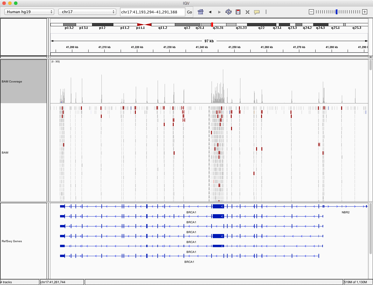
Visualize sequencing depth in IGV
IGV is good for daily research, but when it comes to customization, there aren’t many options. And if the visualization is aimed for publishing, one might want the figure to be vectorized and, more importantly, reproducible.
Therefore, combining with what I learnt in Genomic Data Processing in Bioconductor, I tried to plot the sequencing depth in R with Gviz. I thought learning Gviz will be demanding, since its vignette has 80 pages and the function documentation are scarily long spells. But both of them turned out to be really helpful and informative, especially when trying to tune its behavior. Figures produced by Gviz are aesthetically pleasing, and Gviz has many features as well (still trying). I’m glad that I gave it a shot.
If you want to follow the code yourself, any human BAM alignment files will do. For example, the GEO dataset GSE48215 contains exome sequencing of breast cancer cell lines.
Convert sequencing depth to BedGraph format
After a quick search, Gviz’s DataTrack accepts BedGraph format. This format can display any numerical value of chromosome ranges, shown as follows,
| chromosome | start | end | value |
|---|---|---|---|
| chr1 | 10,051 | 10,093 | 2 |
| chr1 | 10,093 | 10,104 | 5 |
| … | … | … | … |
So we need to convert the alignment result as BedGraph format, which can be done by BEDTools’ genomecov command. On BEDTools’ documentation, it notes that the BAM file should be sorted.
bedtools genomecov -bg -ibam myseq.bam > myseq.bedGraph
The plain text BedGraph can be huge, pipe’d with gzip will reduce file size to around 30% of the original.
bedtools genomecov -bg -ibam myseq.bam | gzip > myseq.bedGraph.gz
Plot depth in Gviz
R packages of human genome annotations (Homo.sapiens) and Gviz itself are required. Also, data.table gives an impressed speed at reading text tables so is recommended to use. During the analysis, I happened to know that data.table supports reading gzip’d file through pipe, which makes it more awesome.
First Gviz track
We should first start at reading our sequencing depth as BedGraph format and plot it.
library(data.table)
library(Gviz)

bedgraph_dt <- fread(
    './coverage.bedGraph',
    col.names = c('chromosome', 'start', 'end', 'value')
)

# Specifiy the range to plot
thechr <- "chr17"
st <- 41176e3
en <- 41324e3

bedgraph_dt_one_chr <- bedgraph_dt[chromosome == thechr]
dtrack <- DataTrack(
    range = bedgraph_dt_one_chr,
    type = "a",
    genome = 'hg19',
    name = "Seq. Depth"
)
plotTracks(
    list(dtrack),
    from = st, to = en
)
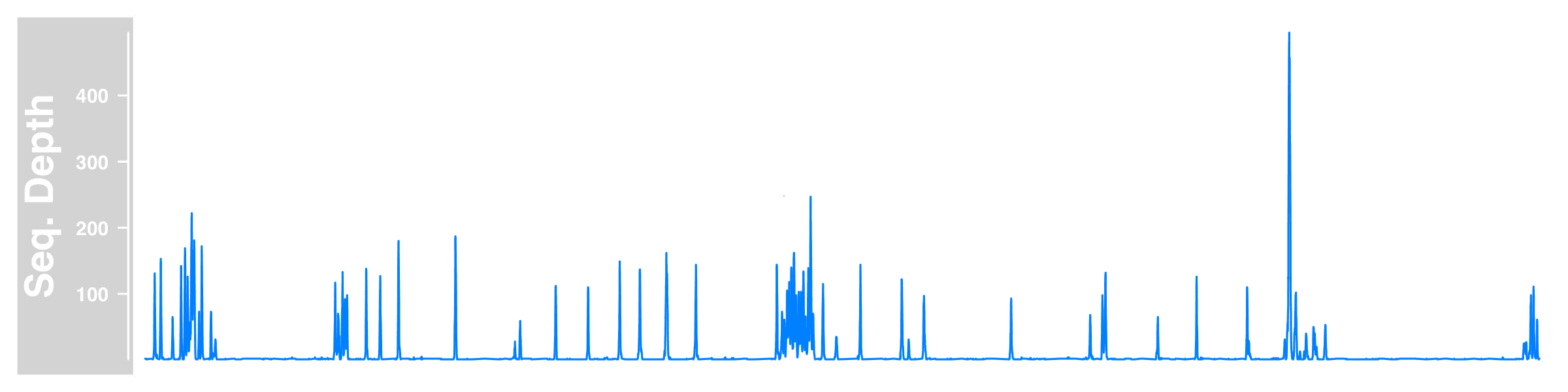
So we read the sequencing depth data, create a Gviz DataTrack holding the subset of our data on chr17, then plot Gviz tracks by plotTracks (though we only made one here) within a given chromosome region. Here is what we got.
Add genome axis
The figure is a bit weird and lack of information without the genomic location.
Adding genomic location can be done automatically by Gviz through a new track GenomeAxisTrack. Also, we’d like to show which region of chromosome we are at. This can be done by adding another track, IdeogramTrack, to show the chromosome ideogram. Note that the latter track will download cytoband data from UCSC so the given genome must have a valid name.
itrack <- IdeogramTrack(
    genome = "hg19", chromosome = thechr
)
gtrack <- GenomeAxisTrack()

plotTracks(
    list(itrack, gtrack, dtrack),
    from = st, to = en
)
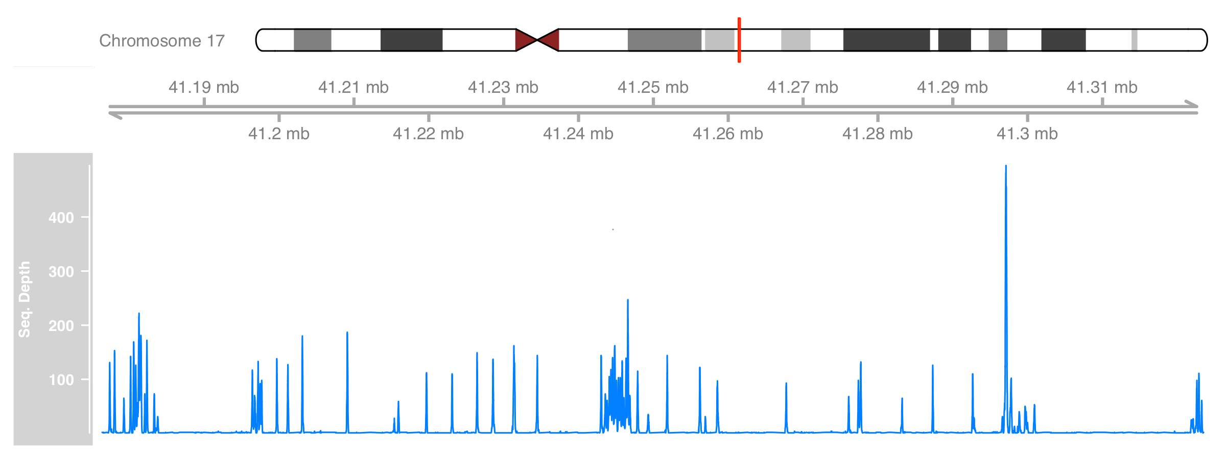
Better now :)
Add annotation
Since we are using exome sequencing, the curve of sequencing depth only makes senses when combined with the transcript annotations.
Gviz has GeneRegionTrack to extract annotation from the R annotation packages. Package Homo.sapiens includes the gene annotation package using UCSC knownGene database. Adding this new track and we will have annotation on our plot.
library(TxDb.Hsapiens.UCSC.hg19.knownGene)
txdb <- TxDb.Hsapiens.UCSC.hg19.knownGene

grtrack <- GeneRegionTrack(
    txdb,
    chromosome = thechr, start = st, end = en,
    showId = TRUE,
    name = "Gene Annotation"
)

plotTracks(
    list(itrack, gtrack, dtrack, grtrack),
    from = st, to = en
)
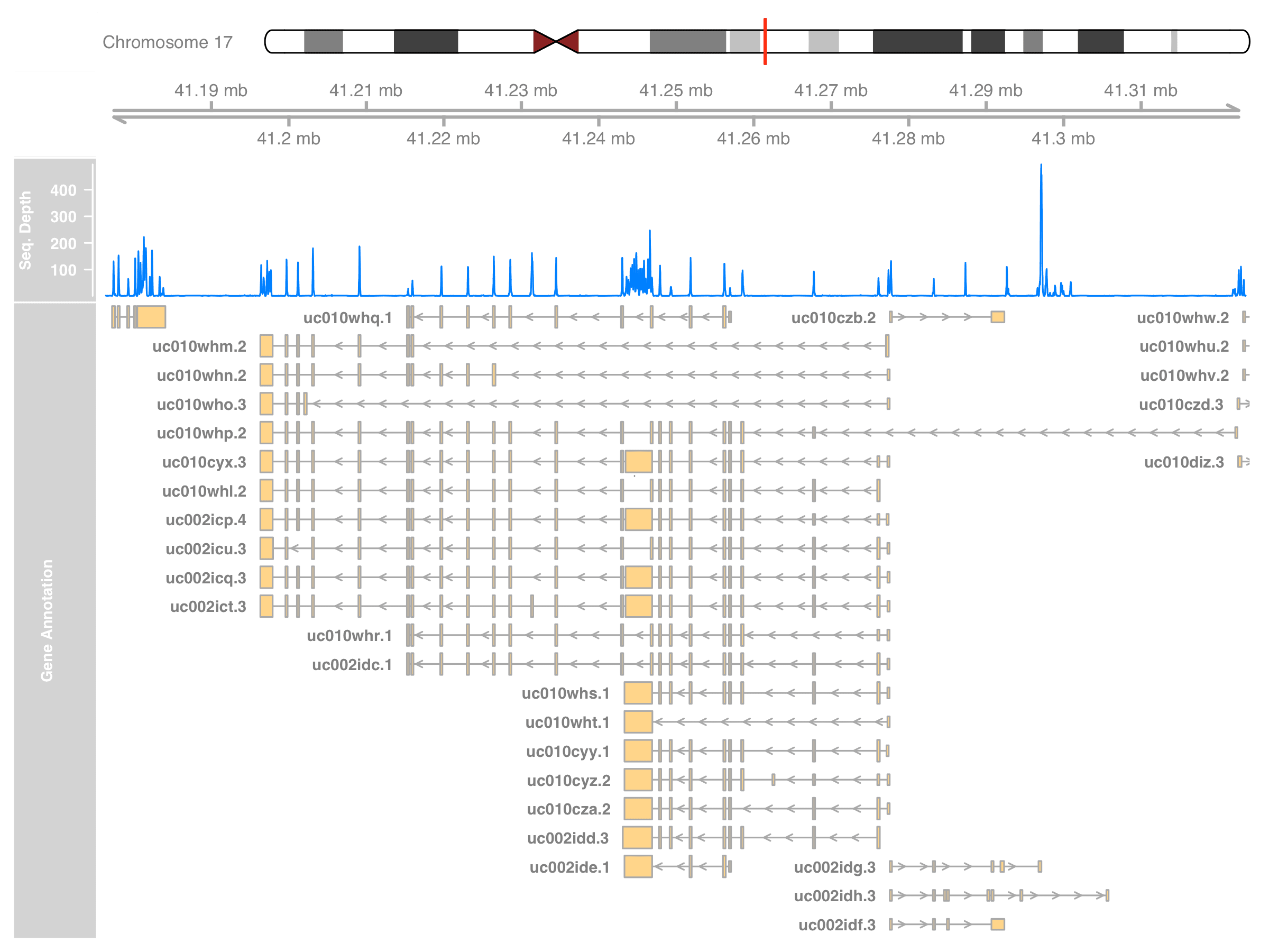
The plot should now be as informative as what we can get from the IGV. In fact, Gviz can plot the alignment result too. It can read the BAM file directly and show a more detailed coverage that matches what IGV can do. I’ll leave that part at the end of this post.
So far we’ve shown the sequencing depth of some chromosome region with annotation. However, there still leave something to be desired, mostly about the annotation:
- Can we show only the annotation of certain genes?
- knownGene’s identifier is barely meaningless, can we show the gene symbol instead?
So here comes the second part, annotation fine tuning.
Plot fine tune
Say, we only care about gene BRCA1. So we need to get its location, or specifically, the genomic range that cover all BRCA1 isoforms. In the following example, I will demonstrate the Gviz’s annotation fine tuning.
Genome annotation query in Bioconductor/R
If you are not familiar with how to query annotations in Bioconductor, it’s easier to think by breaking our goal of finding BRCA1’s ranges into two steps:
- Get the transcript IDs
- Query the transcript locations by their IDs
Getting transcript IDs given their gene symbol is a select() on OrganismDb object,
# Get all transcript IDs of gene BRCA1
BRCA1_txnames <- select(
    Homo.sapiens,
    keys = "BRCA1", keytype = "SYMBOL",
    columns = c("ENTREZID", "TXNAME")
)$TXNAME
> BRCA1_txnames
 [1] "uc010whl.2" "uc002icp.4" "uc010whm.2" "uc002icu.3"
 [5] "uc010cyx.3" "uc002icq.3" "uc002ict.3" "uc010whn.2"
 [9] "uc010who.3" "uc010whp.2" "uc010whq.1" "uc002idc.1"
[13] "uc010whr.1" "uc002idd.3" "uc002ide.1" "uc010cyy.1"
[17] "uc010whs.1" "uc010cyz.2" "uc010cza.2" "uc010wht.1"
Look like it has plenty of isoforms!
via transcripts()
For the transcript location, the easiest way will be querying the txDb via transcript(),
BRCA1_txs <- transcripts(
    Homo.sapiens,
    vals=list(tx_name = BRCA1_txnames),
    columns=c("TXNAME","SYMBOL", "EXONID")
)
> BRCA1_txs
GRanges object with 20 ranges and 3 metadata columns:
       seqnames               ranges strand   |                   EXONID          TXNAME          SYMBOL
          <Rle>            <IRanges>  <Rle>   |            <IntegerList> <CharacterList> <CharacterList>
   [1]    chr17 [41196312, 41276132]      -   | 227486,227485,227482,...      uc010whl.2           BRCA1
   [2]    chr17 [41196312, 41277340]      -   | 227487,227486,227485,...      uc002icp.4           BRCA1
   [3]    chr17 [41196312, 41277340]      -   | 227487,227464,227463,...      uc010whm.2           BRCA1
   [4]    chr17 [41196312, 41277468]      -   | 227489,227486,227485,...      uc002icu.3           BRCA1
   [5]    chr17 [41196312, 41277468]      -   | 227489,227486,227482,...      uc010cyx.3           BRCA1
   ...      ...                  ...    ... ...                      ...             ...             ...
  [16]    chr17 [41243452, 41277340]      -   | 227487,227486,227485,...      uc010cyy.1           BRCA1
  [17]    chr17 [41243452, 41277468]      -   | 227489,227486,227485,...      uc010whs.1           BRCA1
  [18]    chr17 [41243452, 41277500]      -   | 227488,227486,227485,...      uc010cyz.2           BRCA1
  [19]    chr17 [41243452, 41277500]      -   | 227488,227486,227485,...      uc010cza.2           BRCA1
  [20]    chr17 [41243452, 41277500]      -   |            227488,227474      uc010wht.1           BRCA1
  -------
  seqinfo: 93 sequences (1 circular) from hg19 genome
Then get the genomic range of these transcripts by seqnames(), start() and end() functions on the GRanages object,
thechr <- as.character(unique(
    seqnames(BRCA1_txs)
))
st <- min(start(BRCA1_txs)) - 2e4
en <- max(end(BRCA1_txs)) + 1e3
Some space are added at both ends so the plot won’t tightly fit all transcripts and leave some room for the transcript names.
> c(thechr, st, en)
[1] "chr17"    "41176312" "41323420"
via exonsBy()
Another way to obtain the genomic range is getting the exact range of CDS (e.g. exons and UTRs) for each transcript via exonsBy().
BRCA1_cds_by_tx <- exonsBy(
    Homo.sapiens, by="tx", use.names=TRUE
)[BRCA1_txnames]
The function returns a GRangesList object, a list of GRanges that each GRanges object corresponds to a transcript respectively.
> BRCA1_cds_by_tx
GRangesList object of length 20:
$uc010whl.2
GRanges object with 22 ranges and 3 metadata columns:
       seqnames               ranges strand   |   exon_id   exon_name exon_rank
          <Rle>            <IRanges>  <Rle>   | <integer> <character> <integer>
   [1]    chr17 [41276034, 41276132]      -   |    227486        <NA>         1
   [2]    chr17 [41267743, 41267796]      -   |    227485        <NA>         2
   [3]    chr17 [41258473, 41258550]      -   |    227482        <NA>         3
   [4]    chr17 [41256885, 41256973]      -   |    227481        <NA>         4
   [5]    chr17 [41256139, 41256278]      -   |    227480        <NA>         5
   ...      ...                  ...    ... ...       ...         ...       ...
  [18]    chr17 [41209069, 41209152]      -   |    227462        <NA>        18
  [19]    chr17 [41203080, 41203134]      -   |    227461        <NA>        19
  [20]    chr17 [41201138, 41201211]      -   |    227459        <NA>        20
  [21]    chr17 [41199660, 41199720]      -   |    227458        <NA>        21
  [22]    chr17 [41196312, 41197819]      -   |    227457        <NA>        22

...
<19 more elements>
-------
seqinfo: 93 sequences (1 circular) from hg19 genome
GRangesList is not merely a R list structure, which can correctly propagate the GRanges-related functions to all the GRanges it contain.
> start(BRCA1_cds_by_tx)
IntegerList of length 20
[["uc010whl.2"]] 41276034 41267743 41258473 ... 41201138 41199660 41196312
[["uc002icp.4"]] 41277199 41276034 41267743 ... 41201138 41199660 41196312
...
Here we only cares about the widest range, so the hierarchical structure is not useful. It would be better to flatten the GRangesList first,
> BRCA1_cds_flatten <- unlist(BRCA1_cds_by_tx)
> BRCA1_cds_flatten
GRanges object with 284 ranges and 3 metadata columns:
             seqnames               ranges strand   |   exon_id   exon_name exon_rank
                <Rle>            <IRanges>  <Rle>   | <integer> <character> <integer>
  uc010whl.2    chr17 [41276034, 41276132]      -   |    227486        <NA>         1
  uc010whl.2    chr17 [41267743, 41267796]      -   |    227485        <NA>         2
  uc010whl.2    chr17 [41258473, 41258550]      -   |    227482        <NA>         3
  uc010whl.2    chr17 [41256885, 41256973]      -   |    227481        <NA>         4
  uc010whl.2    chr17 [41256139, 41256278]      -   |    227480        <NA>         5
         ...      ...                  ...    ... ...       ...         ...       ...
  uc010cza.2    chr17 [41249261, 41249306]      -   |    227477        <NA>         7
  uc010cza.2    chr17 [41247863, 41247939]      -   |    227476        <NA>         8
  uc010cza.2    chr17 [41243452, 41246877]      -   |    227474        <NA>         9
  uc010wht.1    chr17 [41277288, 41277500]      -   |    227488        <NA>         1
  uc010wht.1    chr17 [41243452, 41246877]      -   |    227474        <NA>         2
  -------
  seqinfo: 93 sequences (1 circular) from hg19 genome
We have the BRCA1 genomic region, rest of the plotting is the same.
Show only the annotations of certain genes
Before we start to create our own annotation subset, we first take a look at what Gviz generated. The GeneRegionTrack track store its annotation data at slot range.
> grtrack@range
GRanges object with 459 ranges and 7 metadata columns:
        seqnames               ranges strand   |     feature          id         exon  transcript        gene      symbol   density
           <Rle>            <IRanges>  <Rle>   | <character> <character>  <character> <character> <character> <character> <numeric>
    [1]    chr17 [41177258, 41177364]      +   |        utr5     unknown uc002icn.3_1  uc002icn.3        8153  uc002icn.3         1
    [2]    chr17 [41177365, 41177466]      +   |         CDS     unknown uc002icn.3_1  uc002icn.3        8153  uc002icn.3         1
    [3]    chr17 [41177977, 41178064]      +   |         CDS     unknown uc002icn.3_2  uc002icn.3        8153  uc002icn.3         1
    [4]    chr17 [41179200, 41179309]      +   |         CDS     unknown uc002icn.3_3  uc002icn.3        8153  uc002icn.3         1
    [5]    chr17 [41180078, 41180212]      +   |         CDS     unknown uc002icn.3_4  uc002icn.3        8153  uc002icn.3         1
    ...      ...                  ...    ... ...         ...         ...          ...         ...         ...         ...       ...
  [455]    chr17 [41277294, 41277468]      -   |        utr5     unknown uc010cyx.3_1  uc010cyx.3         672  uc010cyx.3         1
  [456]    chr17 [41277294, 41277468]      -   |        utr5     unknown uc002idc.1_1  uc002idc.1         672  uc002idc.1         1
  [457]    chr17 [41277294, 41277468]      -   |        utr5     unknown uc010whr.1_1  uc010whr.1         672  uc010whr.1         1
  [458]    chr17 [41277294, 41277468]      -   |        utr5     unknown uc010whs.1_1  uc010whs.1         672  uc010whs.1         1
  [459]    chr17 [41322143, 41322420]      -   |        utr5     unknown uc010whp.2_1  uc010whp.2         672  uc010whp.2         1
  -------
  seqinfo: 1 sequence from hg19 genome; no seqlengths
So we filter out unrelated ranges by checking if the value of metadata column transcript is one of BRCA1’s transcript IDs,
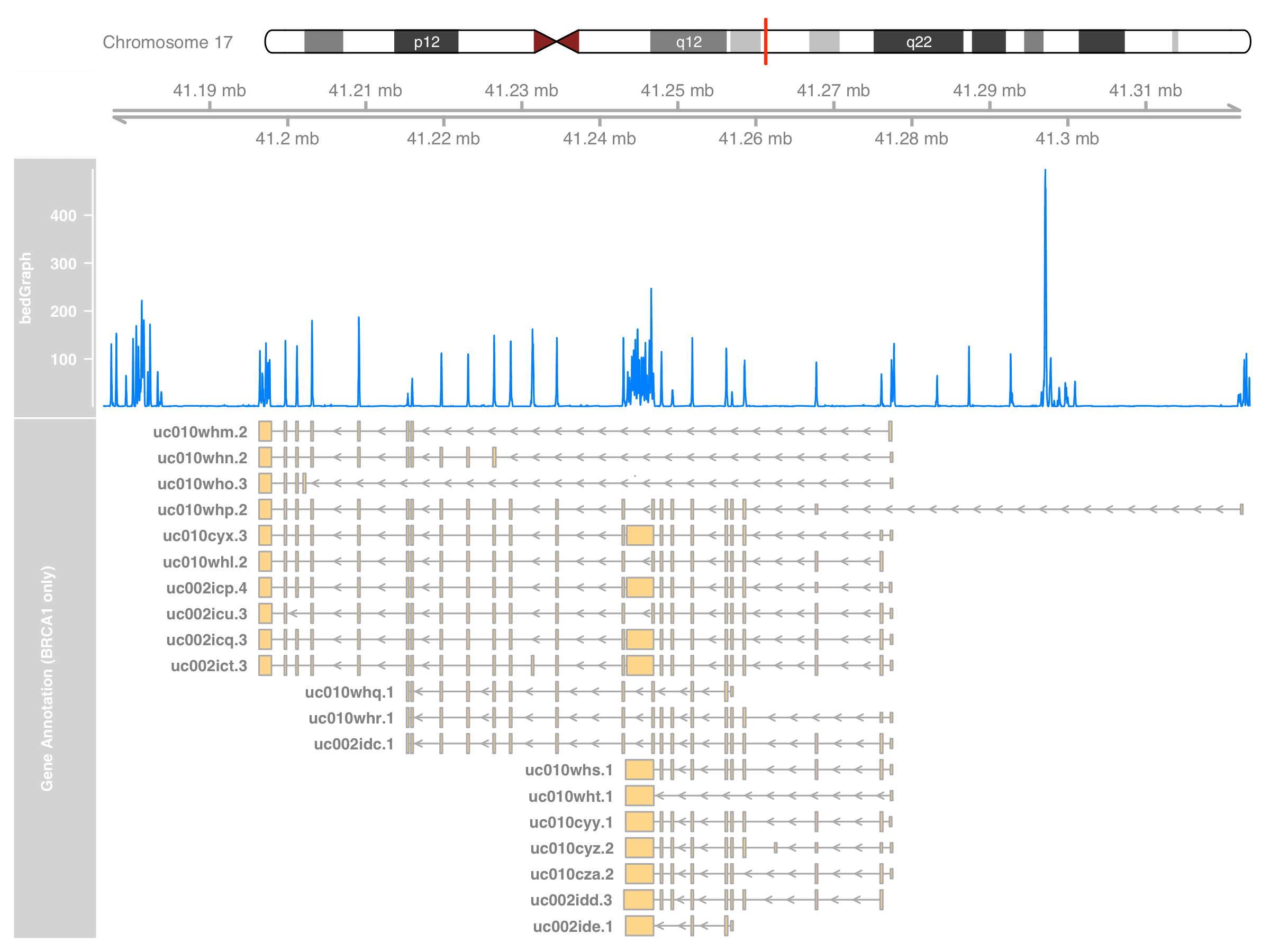
BRCA_only_range <- grtrack@range[
    mcols(grtrack@range)$transcript %in% BRCA1_txnames
]
grtrack@range <- BRCA_only_range
or by less hacky way that use the new range to construct another GeneRegionTrack,
grtrack_BRCA_only <- GeneRegionTrack(
    BRCA_only_range,
    chromosome = thechr, start = st, end = en,
    showId = TRUE,
    name = "Gene Annotation (BRCA1 only)"
)
plotTracks(
    list(itrack, gtrack, dtrack, grtrack_BRCA_only),
    from = st, to = en
)
Display gene symbols at annotation track
It’s more obvious now about how Gviz stores the annotation. All we need is to replace the symbol name with whatever we desire.
First, we extract the metadata of the GeneRegionTrack, and query for their gene symbols. Using either the transcript ID or Entrez ID will do.
grtrack_range <- grtrack@range
range_mapping <- select(
    Homo.sapiens,
    keys = mcols(grtrack_range)$symbol,
    keytype = "TXNAME",
    columns = c("ENTREZID", "SYMBOL")
)
> head(range_mapping)
      TXNAME SYMBOL ENTREZID
1 uc002icn.3   RND2     8153
2 uc002icn.3   RND2     8153
3 uc002icn.3   RND2     8153
4 uc002icn.3   RND2     8153
5 uc002icn.3   RND2     8153
6 uc002icn.3   RND2     8153
Then we concatenate the information of transcript ID and gene symbol using stringr.
library(stringr)
new_symbols <- with(
    range_mapping,
    str_c(SYMBOL, " (", TXNAME, ")", sep = "")
)
> head(unique(new_symbols))
[1] "RND2 (uc002icn.3)" "NBR2 (uc002idf.3)" "NBR2 (uc010czb.2)"
[4] "NBR2 (uc002idg.3)" "NBR2 (uc002idh.3)" "NBR1 (uc010czd.3)"
Like how we extract BRCA1-only annotations, we construct a new GeneRegionTrack.
grtrack_symbol <- GeneRegionTrack(
    grtrack@range,
    chromosome = thechr, start = st, end = en,
    showId = TRUE,
    name = "Gene Annotation w. Symbol"
)
symbol(grtrack_symbol) <- new_symbols
plotTracks(
    list(itrack, gtrack, dtrack, grtrack_symbol),
    from = st, to = en
)
Summary
So we’ve learnt how to plot using Gviz. You should go explore other data tracks or try to combine sequencing depth of multiple samples. I found the design of Gviz is clean and easy to modify. I think I’ll use Gviz whenever genome-related plots are needed.
Really glad I’ve tried it :)
Supplementary - Plot BAM files directly
We will start by replacing DataTrack with AlignmentsTrack. Also we select a smaller region this time so the read mapping can be clearly seen.
st <- 41.196e6L
en <- 41.202e6L
gtrack <- GenomeAxisTrack(cex = 1)  # set the font size larger
altrack <- AlignmentsTrack(
    "myseq.bam", isPaired = TRUE, col.mates = "deeppink"
)
plotTracks(
    list(gtrack, altrack, grtrack),
    from = st, to = en
)
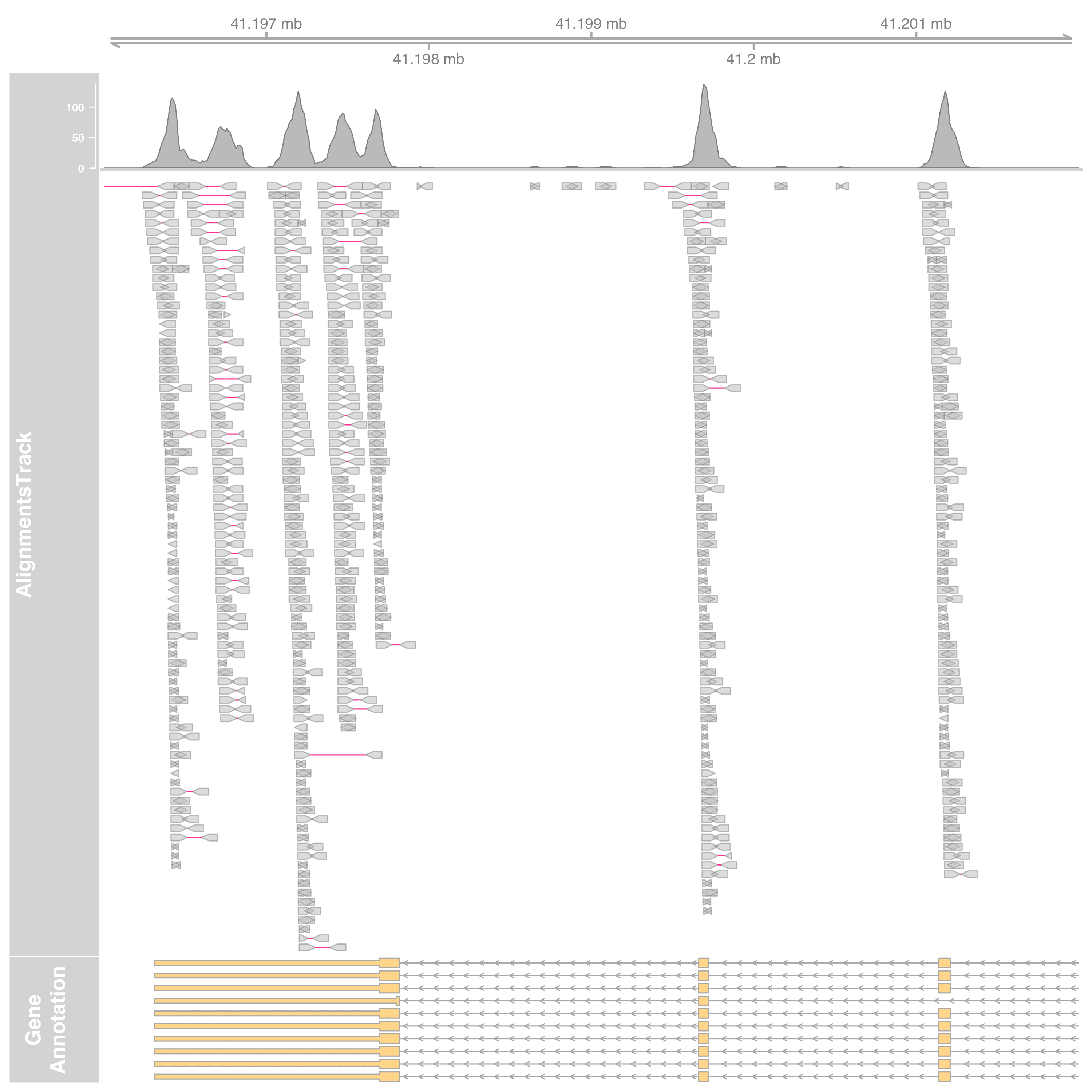
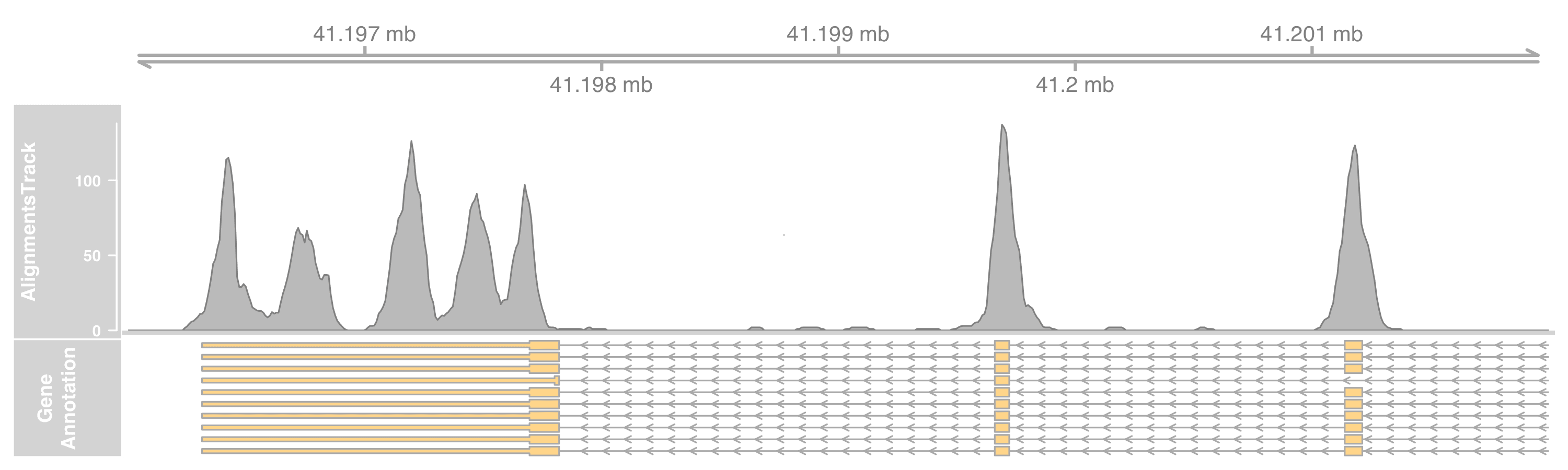
To plot only the coverage, set the type as coverage.
altrack <- AlignmentsTrack(
    "myseq.bam", type = "coverage"
)
Fancier alignment display
Spend some time reading the documentation, the alignment can be much more fancier.
For example, when looking at a much smaller genome region, we many want to see the sequence and read mismatches. It could be done by adding a new track SequenceTrack to include the genome sequence,
small_st <- 41267.735e3L
small_en <- 41267.805e3L

library(BSgenome.Hsapiens.UCSC.hg19)
strack <- SequenceTrack(
    Hsapiens,
    chromosome = thechr, from = small_en, to = small_st,
    cex=0.8
)
We tweak other tracks as well to make sure the figure won’t explode by too much information. Gene annotations are collapsed down to one liner. Also, aligned read’s height is increased to fit in individual letters (e.g., ATCG).
grtrack_small <- GeneRegionTrack(
   grtrack@range,
   chromosome = thechr,
   start = small_st, end = small_en,
   stacking = "dense",
   name = "Gene Annotation"
)
altrack <- AlignmentsTrack(
    "myseq.bam",
    isPaired = TRUE,
    min.height = 12, max.height = 15, coverageHeight = 0.15, size = 50
)
plotTracks(
    list(gtrack, altrack, grtrack_small, strack),
    from = small_st, to = small_en
)
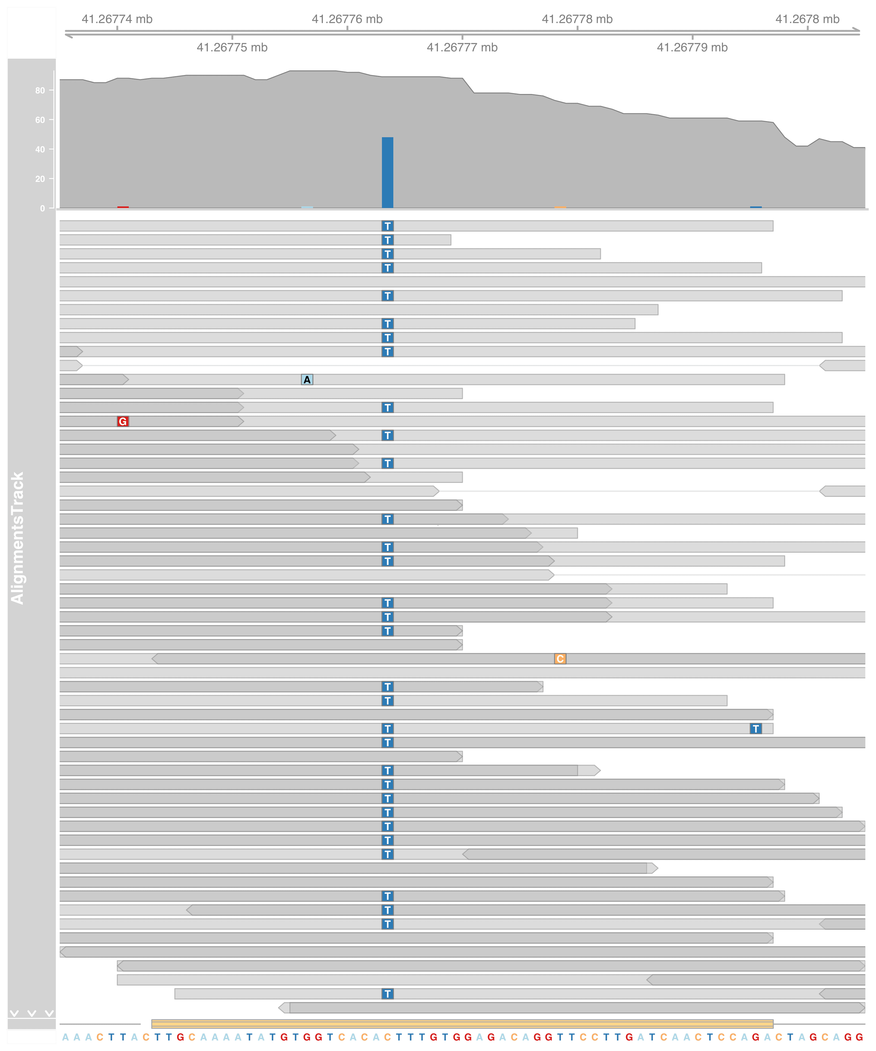
We found a C>T SNP here!