This is not a tutorial.
The goal of this talk is to introduce the related packages and provide some keywords for each task.
Since it is going to cover a lot of different topics, this talk assumes the reader has the basic understanding of:
R; familiar with the main topics mentioned in R for Data Science (a great entry-level book)
Pipe operators (|> or %>%); see below
tidyverse packages (readr, dplyr, purrr, ggplot2)
grid graphics (mostly gpar(...) parameters)
Since R 4.1, R introduces a native pipe operator |>.
For example, the following code are equivalent:
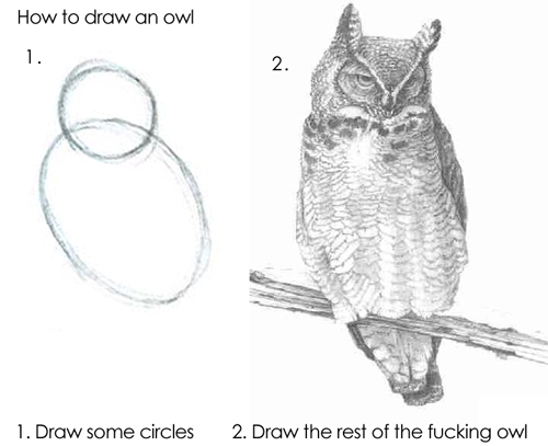
To many people (including me), there will steps in the instructions as large as the ones in "how to draw an owl" in the slides.
This is intentional, because I don't want to cover all the technical details in this talk.
There are far better in-depth tutorials and guides for each package and topic.
I will provide links to those materials in the slides and the slide notes.
I hope today we can all know the tools and directions, then draw the basic circles of the owl 🦉.
Our goal
About me
PhD in Computational and Systems Biology
from Washington University in St. Louis
Thesis research: cancer proteogenomics (analysis and tool/pipeline development)
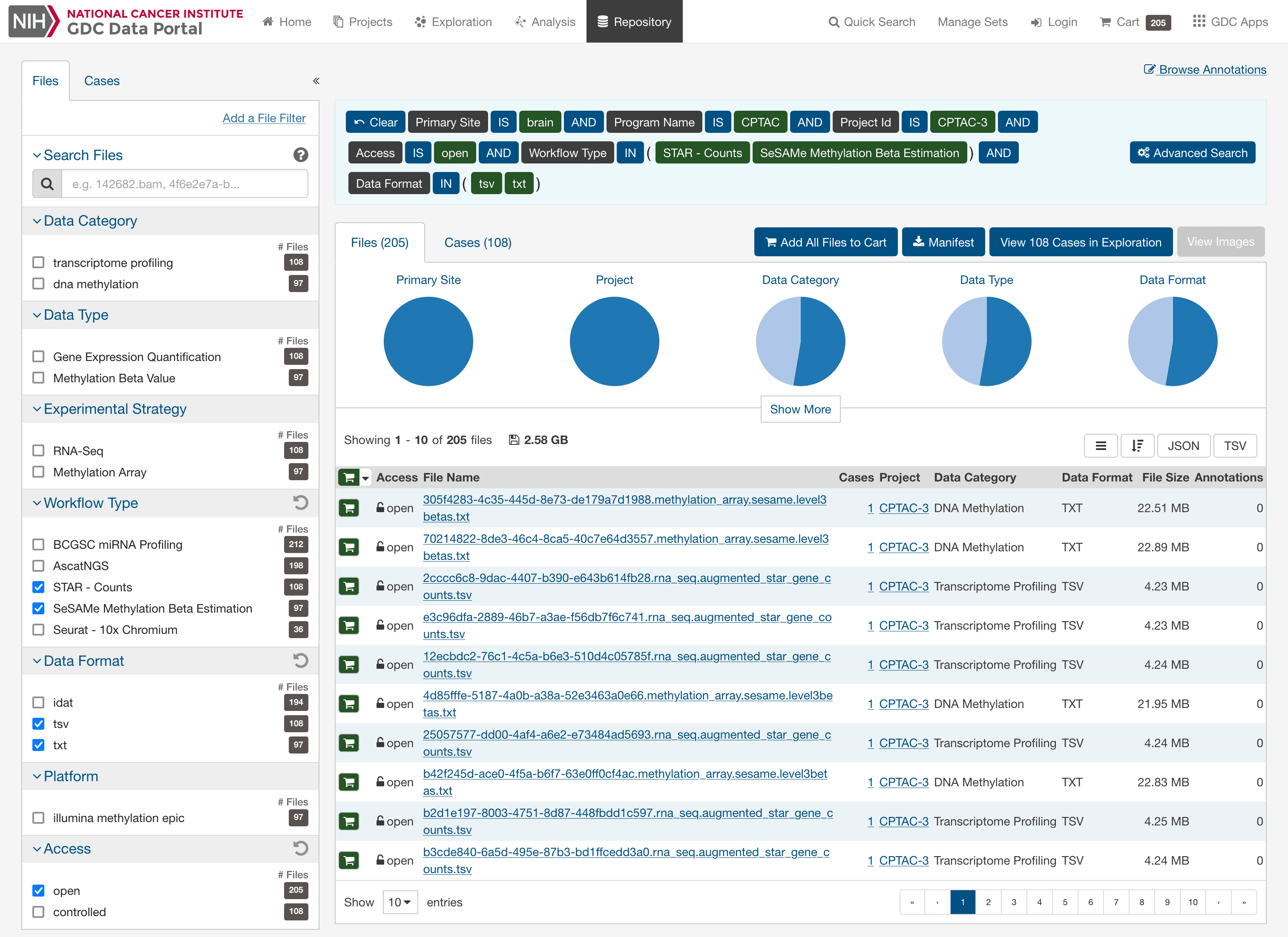
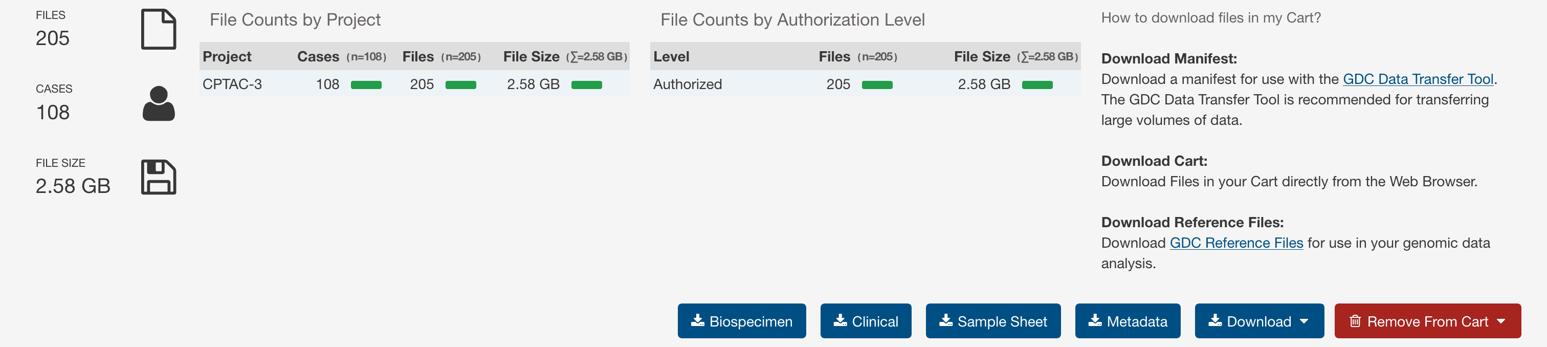
Worked in related consortia including
CPTAC,
TCGA,
and HTAN with thousands of samples
Background knowledge about genomics
Genome (DNA) = source code of our cells
If we measure DNA/RNA/protein/...,
we know what's going on in a cell (?)
High-throughput technologies enable us to capture cell-wide/genome-wide signals
(DNA-seq, RNA-seq, microarray, mass spectrometry, imaging, ...)
From external files (BED, GTF, and etc): use rtracklayer package
Good practice: always provide/verify the correct genome information
(Seqinfo object from GenomeInfoDb package)
GenomicRanges provides many methods to manipulate the ranges
# All methods are strand aware
?"intra-range-methods"    # Methods applied to every range independently
shift(), narrow(), flank(), promoters(), resize(), ...

?"inter-range-methods"    # Methods applied across all ranges at once
range(), reduce(), gaps(), disjoin(), coverage(), ...

?"findOverlaps-methods"   # Find overlaps between two ranges
findOverlaps(), countOverlaps(), %over%, %within%, %outside%, ...

methods(class="GRanges")  # List all available methods
GenomeInfoDb is a powerful package for genome information
my blog post to create a Seqinfo object from a genome .dict file.
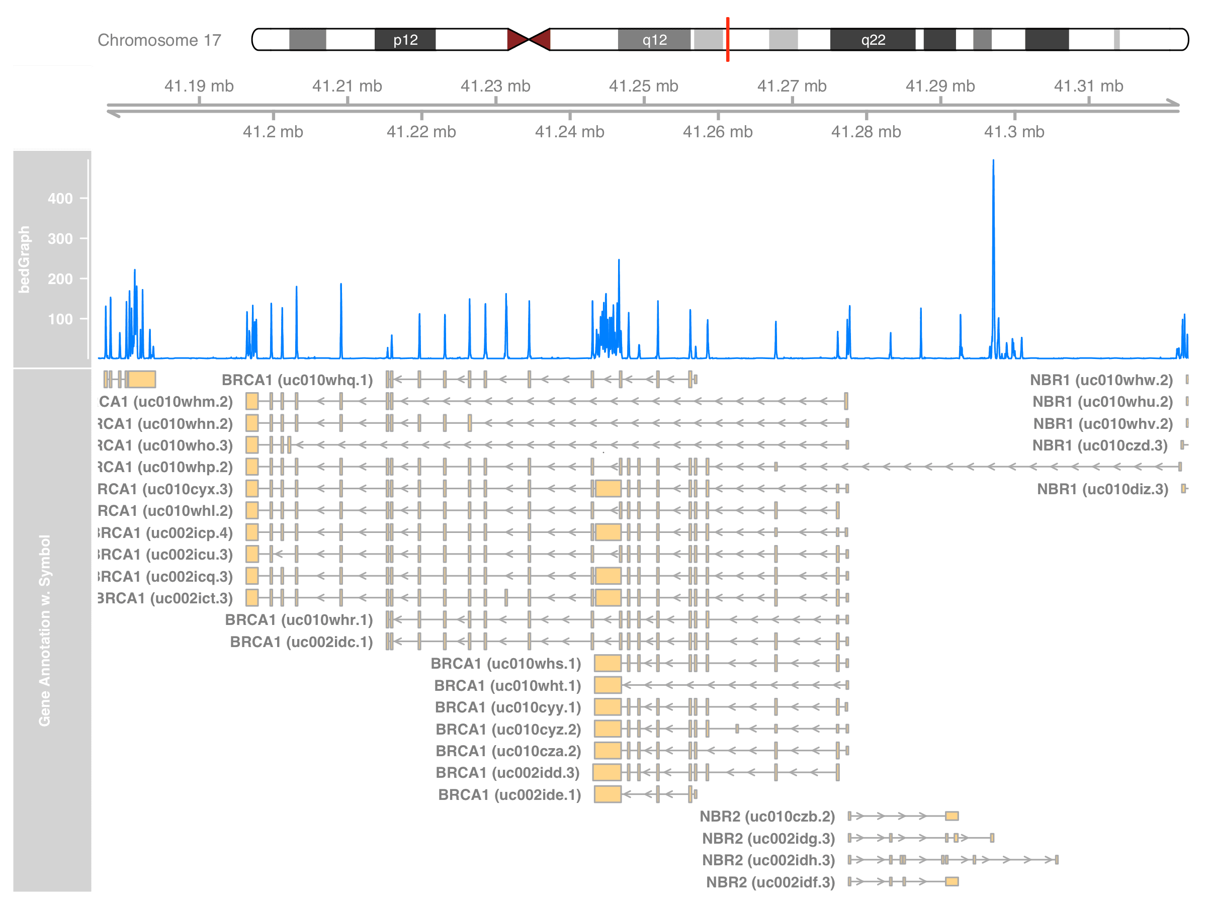
Query genome annotations by ensembldb
Find the location of a genomic feature
ID conversion (gene ↔ transcript ↔ protein)
ensembldb
provides a local copy of Ensembl genome annotations (EnsDb.*)
Fix a certain version of the annotation for a project
All EnsDb objects (different versions and species) are available on
AnnotationHub.
For example, Ensembl release 102 (GENCODE 36) for human is available as AH89180 on AnnotationHub.
Example: Find all the protein coding genes in autosomes
I find tidyverse's verbs easy to learn and use, personally
Bioconductor and tidyverse are two separate ecosystems
Function overrides are common (e.g. select(), filter())
DataFrame (Bioconductor), tibble (tidyverse), data.frame are all different classes with slightly different behaviors (e.g., row names)
Packages like plyranges and tidybulk introduces "verbs" to Bioconductor classes (still an ongoing process)
Function overrides
By default, the import order of the packages leads to different function overrides. Specify the function explicitly, say,
dplyr::select() and AnnotationDbi::filter().
Alternatively, use packages like conflicted to explicitly resolve function conflicts.
Conversion between DataFrame and tibble
One of the main differences is the use of row names. Row names of DataFrame (and other Bioconductor packages) are very useful, while tibble will remove the row names after subsetting and discourage users to use them.
# Tibble to DataFrame (and use one column as rownames)
my_DF = my_tbl |>
	column_to_rownames("rowname_col") |>
	as("DataFrame")
# DataFrame to tibble (and extract rownames to one column)
my_tbl = my_DF |>
	as_tibble(rownames = "rowname_col")
purrr's map functions are handy to process many samples in the same way
My common use case: read the specific format of a pipeline output for all samples
purrr provides a consistent interface to eliminate most for-loops:
my_list |> map(my_fun): the most basic form
my_list |> imap(...):
also pass the list key/name to the function
my_df |> pmap(function(col_A, col_B){ ... }):
map a data frame of parameters as input
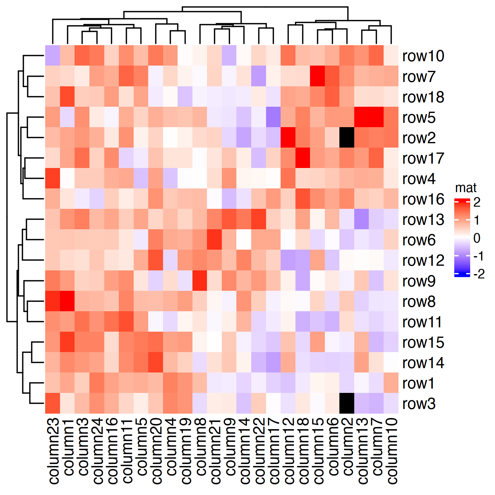
mat = matrix(..., nr = 18, nc = 24)  # see notes

# 1. Define a color mapping function
col_fun = circlize::colorRamp2(
	c(-2, 0, 2), c("blue", "white", "red"))
col_fun(0:3)
# "#FFFFFFFF" "#FF9E81FF" "#FF0000FF" "#FF0000FF"

# 2. Construct the heatmap
ht = Heatmap(
    mat, name = "mat",
    col = col_fun,
    na_col = "black"  # color for NAs
)
draw(ht)
Code to generate the example matrix
The code was copied from the first example in the ComplexHeatmap Complete Reference (Chatper 2: A Single Heatmap).
set.seed(123)
nr1 = 4; nr2 = 8; nr3 = 6; nr = nr1 + nr2 + nr3
nc1 = 6; nc2 = 8; nc3 = 10; nc = nc1 + nc2 + nc3
mat = cbind(
  rbind(
	matrix(rnorm(nr1*nc1, mean = 1, sd = 0.5), nr = nr1),
    matrix(rnorm(nr2*nc1, mean = 0, sd = 0.5), nr = nr2),
  	matrix(rnorm(nr3*nc1, mean = 0, sd = 0.5), nr = nr3)),
  rbind(
	matrix(rnorm(nr1*nc2, mean = 0, sd = 0.5), nr = nr1),
    matrix(rnorm(nr2*nc2, mean = 1, sd = 0.5), nr = nr2),
	matrix(rnorm(nr3*nc2, mean = 0, sd = 0.5), nr = nr3)),
  rbind(
	matrix(rnorm(nr1*nc3, mean = 0.5, sd = 0.5), nr = nr1),
    matrix(rnorm(nr2*nc3, mean = 0.5, sd = 0.5), nr = nr2),
    matrix(rnorm(nr3*nc3, mean = 1, sd = 0.5), nr = nr3))
)
# random shuffle rows and columns
mat = mat[sample(nr, nr), sample(nc, nc)]
# Add column and row names
rownames(mat) = paste0("row", seq_len(nr))
colnames(mat) = paste0("column", seq_len(nc))
# Add some missing values
mat[2:3, 2] = NA_real_
While the color palettes/mappings my_colors can be reused easily in R by exporting it as a RDS file, it's not easy to use from a different language (Python)
# Convert list of color palettes/mappings to a data frame
my_colors_tbl = my_colors |>
    imap_dfr(function(palette, name) {
        palette |>
            enframe('label', 'color') |>
            mutate(column = .env$name)
    }) |>
    select(column, label, color)
# # A tibble: 17 × 3
#   column     label       color
#   <chr>      <chr>       <chr>
# 1 sex        Female      #8700F9
# 2 sex        Male        #00C4AA
# 3 rna        IDH mutant  #2A9C6A
# ...

# Reconstruct the list of color palettes/mappings
# from a exported data frame
my_colors.recovered = my_colors_tbl |>
    split(my_colors_tbl$column) |>
    map(function(data_tbl) {
        data_tbl |>
            select(label, color) |>
            deframe()
    })
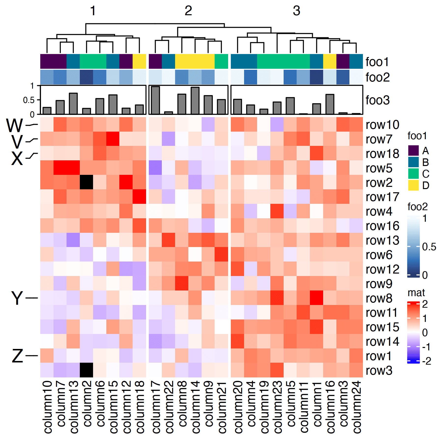
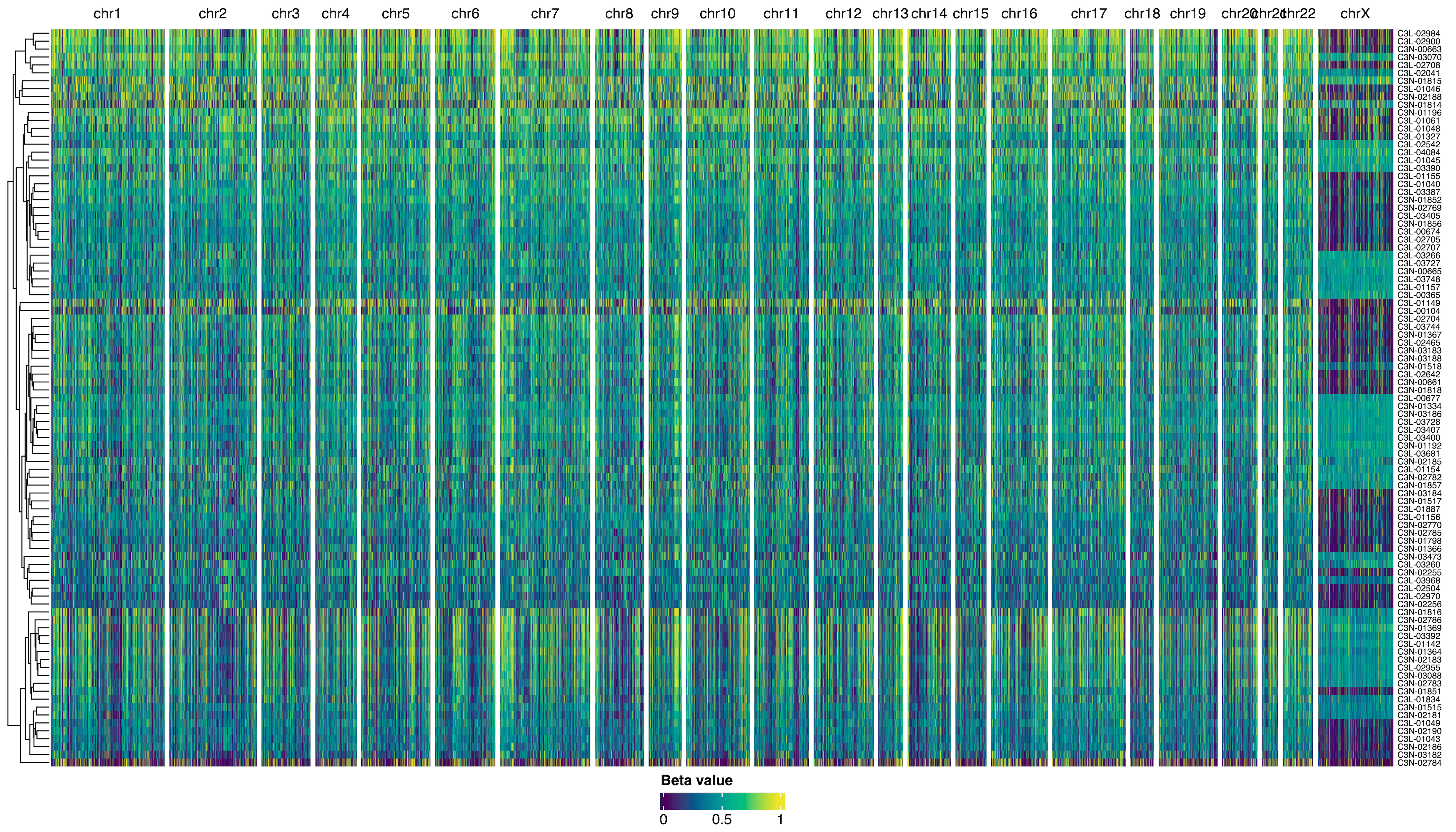
Tips for large heatmaps
Build individual blocks first
Check if all heatmaps and annotations are in the same order
Make heatmap settings reuseable or less automatic
(color palettes, gpar()s, and even dendrograms)


 Our goal


