Genomics in R by Examples
Esc to overview
← → to navigate

Liang-Bo Wang, 2019-03-27.
Liang-Bo Wang
Shared under CC 4.0 BY license
Esc to overview
← → to navigate
Plus all the R packages built on the strong foundation:
Visualization
Statistical analysis
Dataset import
TCGAbiolinksCheck out additional readings for a thorough introduction
install.packages(c(
	"tidyverse",   # dplyr, ggplot2, tibble, stringr, ...
	"BiocManager"  # Bioconductor installer
))
BiocManger::install(c(
	"ensembldb", "EnsDb.Hsapiens.v86",
	"gtrellis", "TCGAbiolinks"
))
EnsDb stores the Ensembl annotation of a specific release of an organism.
library(ensembldb)
library(EnsDb.Hsapiens.v86)
edb <- EnsDb.Hsapiens.v86
ensembldb::select() maps the IDs between columns (keytypes).
ensembldb::select(
    edb,
    keys = c("ENST00000396884"),
    keytype = "TXID",
    columns = c("SYMBOL")
)
#              TXID SYMBOL
# 1 ENST00000396884  SOX10
keytypes(edb)
# ENTREZID
# PROTEINID
# SEQNAME
# SYMBOL
# TXBIOTYPE
# TXID
# ...| Object type | Example packages |
|---|---|
| TxDb |
EnsDb.Hsapiens.v86, TxDb.Hsapiens.UCSC.hg38.knownGene |
| OrgDb | org.Hs.eg.db |
| BSgenome | BSgenome.Hsapiens.UCSC.hg38 |
| Misc. |
Organism.dplyr,
AnnotationHub,
biomaRt, all packages under AnnotationData |
Try another annotation source like org.Hs.eg.db.
biomaRt can convert IDs between different annotation sources.
Use GenomicFeatures::makeTxDbFromGFF to build a new TxDB
from RefSeq's GFF file.
This method applies to all customized GTFs.
			txs <- transcripts(edb, columns = c('symbol')); txs
# GRanges object with 216741 ranges and 1 metadata columns:
#                   seqnames            ranges strand |      symbol
#                      <Rle>         <IRanges>  <Rle> | <character>
#   ENST00000456328        1       11869-14409      + |     DDX11L1
#   ENST00000450305        1       12010-13670      + |     DDX11L1
#   ENST00000488147        1       14404-29570      - |      WASH7P
#               ...      ...               ...    ... .         ...
#   ENST00000435945        Y 26594851-26634652      - |     PARP4P1
#   ENST00000435741        Y 26626520-26627159      - |     FAM58CP
#   ENST00000431853        Y 56855244-56855488      + |     CTBP2P1
#   -------
#   seqinfo: 357 sequences from GRCh38 genome
How to read this output? What is a GRanges object?
GRanges overviewGRanges and GRangesList store genomic ranges in RGRanges cheatsheet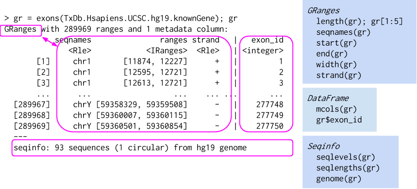
Find the location of all SOX10 transcripts:
txs[txs$symbol == 'SOX10', ]
# GRanges object with 6 ranges and 1 metadata columns:
#                   seqnames            ranges strand |      symbol
#                      <Rle>         <IRanges>  <Rle> | <character>
#   ENST00000446929       22 37970686-37983414      - |       SOX10
#   ENST00000396884       22 37972300-37984537      - |       SOX10
# ...
Calculate their promoter region:
promoters(subset(txs, symbol == 'SOX10'), upstream=2000, downstream=200)
# GRanges object with 6 ranges and 1 metadata columns:
#                   seqnames            ranges strand |      symbol
#                      <Rle>         <IRanges>  <Rle> | <character>
#   ENST00000446929       22 37983215-37985414      - |       SOX10
#   ENST00000396884       22 37984338-37986537      - |       SOX10
# ...
library(rtracklayer)
library(GenomicRanges)
library(gtrellis)
library(EnsDb.Hsapiens.v86)
library(tidyverse)
# Read sequencing depth BED file as a GRanges object
seq_depth_gr <- import.bedGraph('wxs_normal.subset.bed.gz')
# GRanges object with 76574 ranges and 1 metadata column:
# seqnames ranges strand | score
# [1] chr22 23174700-23174716 * | 1
# [2] chr22 23174717-23174725 * | 2
# [3] chr22 23174726-23174735 * | 3
# ...
# Find the genomic range of SOX10
edb <- EnsDb.Hsapiens.v86
seqlevelsStyle(edb) <- 'UCSC'
sox10_region <- range(transcripts(edb, filter = ~ symbol == 'SOX10')) + 500
# GRanges object with 1 range and 0 metadata columns:
# seqnames ranges strand
# [1] chr22 37970186-37987922 -
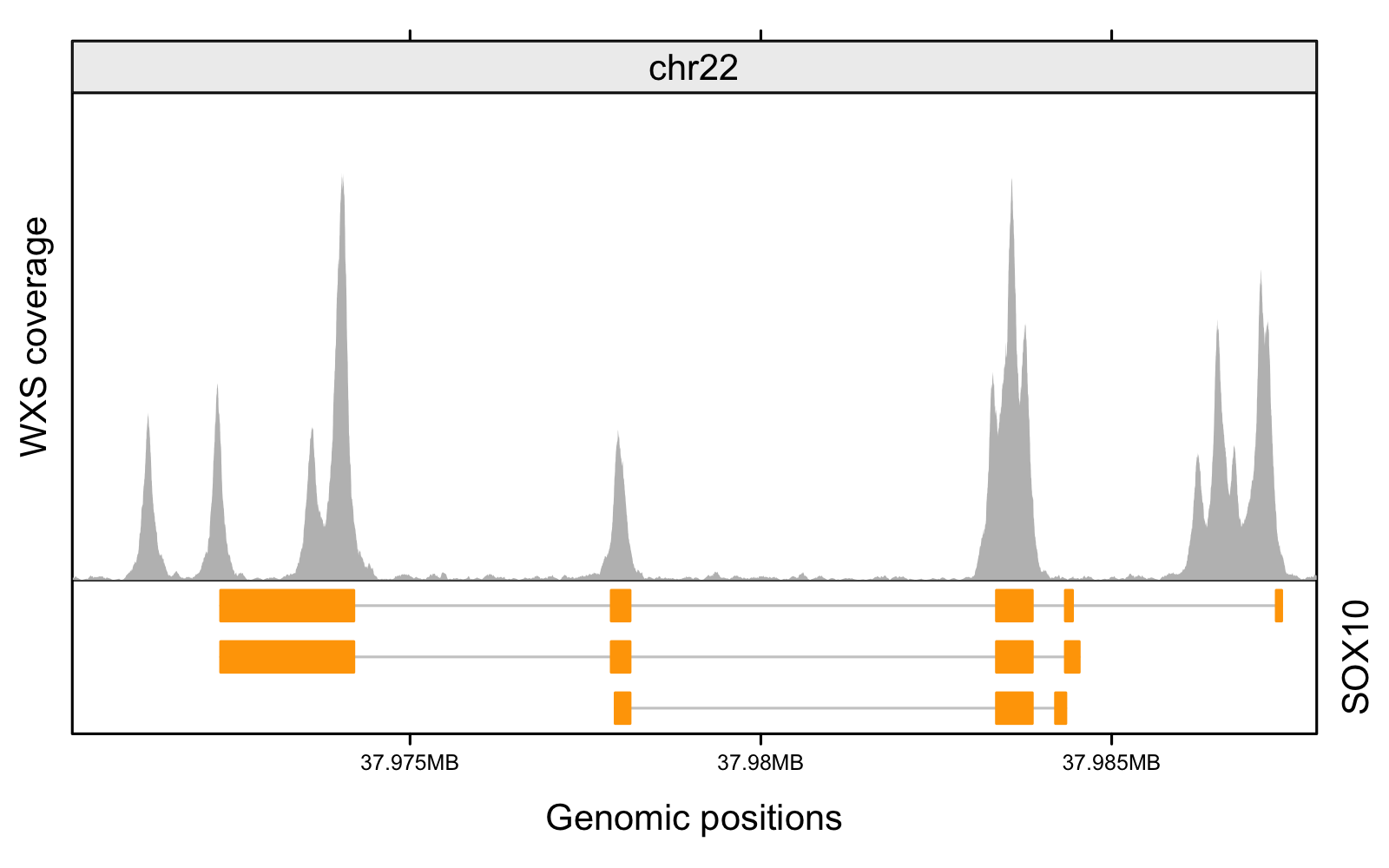
Finally, use gtrellis to plot. gtrellis visualizes tracks of data using chromosomes as x-axis. Useful for CNV, sequencing depths, DNA methylation, and etc.
gtrellis_layout(
    data = sox10_region,  # specify the genomic region of interest
    track_ylim = c(0, 750)
)

# Add the track for WXS sequencing depth
add_lines_track(
    seq_depth_gr,
    seq_depth_gr$score,
    area = TRUE,
    gp = gpar(fill = "gray", col = NA)
)
SummarizedExperiment and RangedSummarizedExperiment
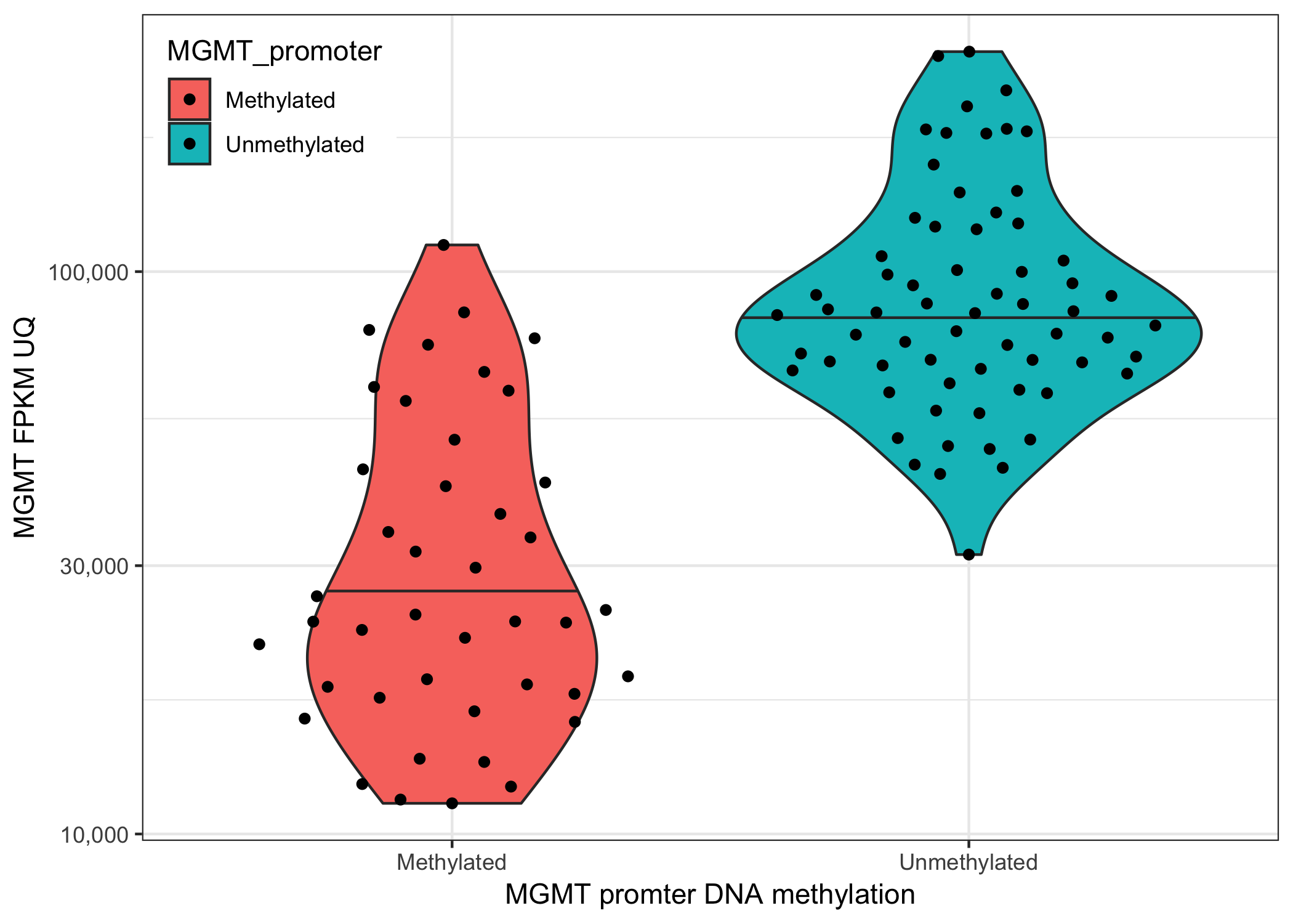
TxDb and EnsDBGRanges and GRangesListgtrellisSummarizedExperimentVisualize the relationship between DNA methylation of MGMT promoter and its gene expression.
SummarizedExperiment objectcolData() to stratify GBM samples by their MGMT methylation status