Convolutional Neural Network From the Ground Up

Liang Bo Wang (亮亮), 2015-05-18

Taiwan R User Group, 2015-05-18

Convolutional Neural Network (CNN) From the Ground Up

Orig. Stanford CS231n course by Andrej Karpathy and
Li Fei-Fei under MIT License

Adapted by Liang2 under CC 4.0 BY license

Esc to overview
to navigate

I don't own / create most of the content

Almost everything are from
Stanford CS231n

Education is the art of conveying a sense of truth by telling a series of decreasing lies.

Steven Wittens, creator of MathBox

Far more details about DNN (CNN) are left out of this talk due to the time constraint. However, you should get the idea how to implement the core parts and be able to read the rest of the materials yourself.

About Me

Supervised Image Classification

  • Input: RGB pixel values
  • Output: classes / labels, usually with a score
  • The classifier learns their relationship from data
  • So data are splitted into training / validation / testing datset

CNN / DL are end-to-end classification

General machine learning framework

  1. A mapping function \(f\) from input features \(x\) to scores of output class \(f\). Class with highest score is chosed as the prediction for input \(i\). $$ \begin{aligned} \hat{y_i} = \arg\max_j f(x_i; W)_j \\ j, y_i \in \{1 \ldots K\} \end{aligned} $$
  2. A loss function \(L\) to compute the difference between \(y_i\) and \(\hat{y_i}\).
  3. Optimize (Lower) the loss by updating the parameter \(W\).
  4. Stop the update when max iterations are reached or stop criteria meets.

Softmax Linear Classification

Linear classifier

Training dataset of images \(x_i \in R^D\) each with label \(y_i\) for \(N\) examples, \(i = 1 \ldots N\) and \(y_i \in 1 \ldots K\). $$f(x_i; W, b) = W x_i + b \quad\quad f: R^D \mapsto R^K$$ where parameters are \(W\) [K x D] called weights and \(b\) [K x 1] called bias vector.

In CIFAR-10 dataset, \(N\) = 50,000, \(D\) = 32 x 32 x 3 = 3072, \(K\) = 10.

Linear classifier visualized

Bias trick

Loss function - Softmax

$$ L_i = -\log\left(\frac{e^{f_{y_i}}}{\sum_j e^{f_j}}\right) $$ \(e^{f_{y_i}}\) is like probability yet being normalized. Ex. \(-\log 10 < -\log 0.01 \). Higher score leads to lower loss.
For numerical stability, in computation \( \frac{e^{f_{y_i}}}{\sum_j e^{f_j}} = \frac{C \cdot e^{f_{y_i}}}{C \cdot \sum_j e^{f_j}} = \frac{e^{f_{y_i} + \log C}}{\sum_j e^{f_j + \log C}} \) and let \( \log C = -\max_j f_j \) to normalized the exp. of the largest score to be 1.

L2 Regularization

Regularization (cont'd)

Loss optimization

Choose the step size (learning rate)

Analytical gradients

Gradient Descent

      # Vanilla Minibatch Gradient Descent
while it < max_iter:
    data_batch = sampling(data, 256)
    dw = gradient(loss_fun, data_batch, w)
    w += - step_size * w
      

Stochastic Gradient Descent (SGD) when batch contains only 1 sample.

Get our hands wet

For what does the CIFAR-10 dataset look like and data preprocessing, try ænotebook 00.

For softmax linear classifier, try notebook 01.

Fully Connected
Neural Network

Our "artifact" neuron as a linear classifier

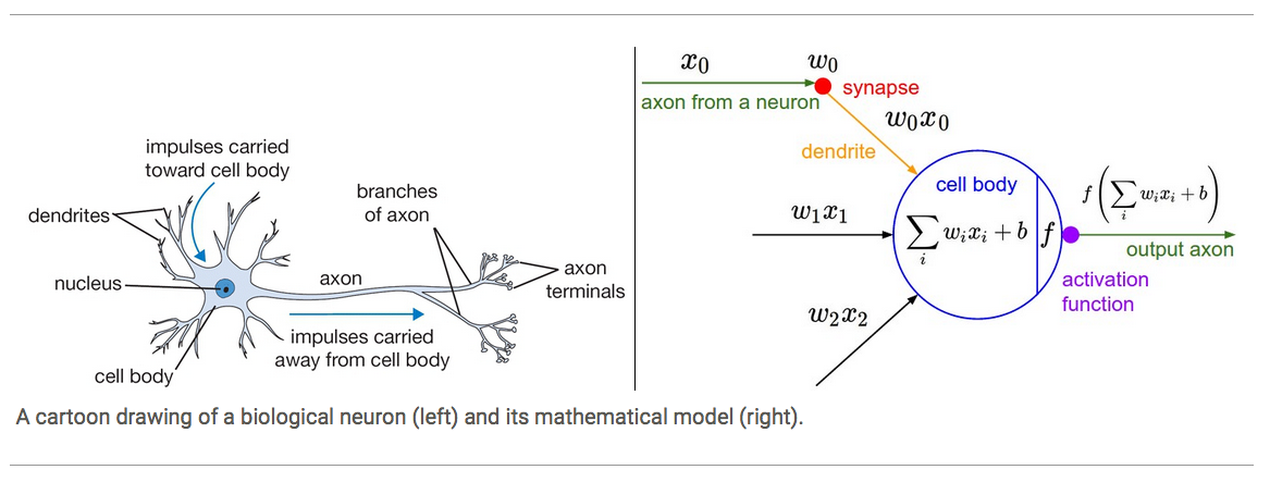
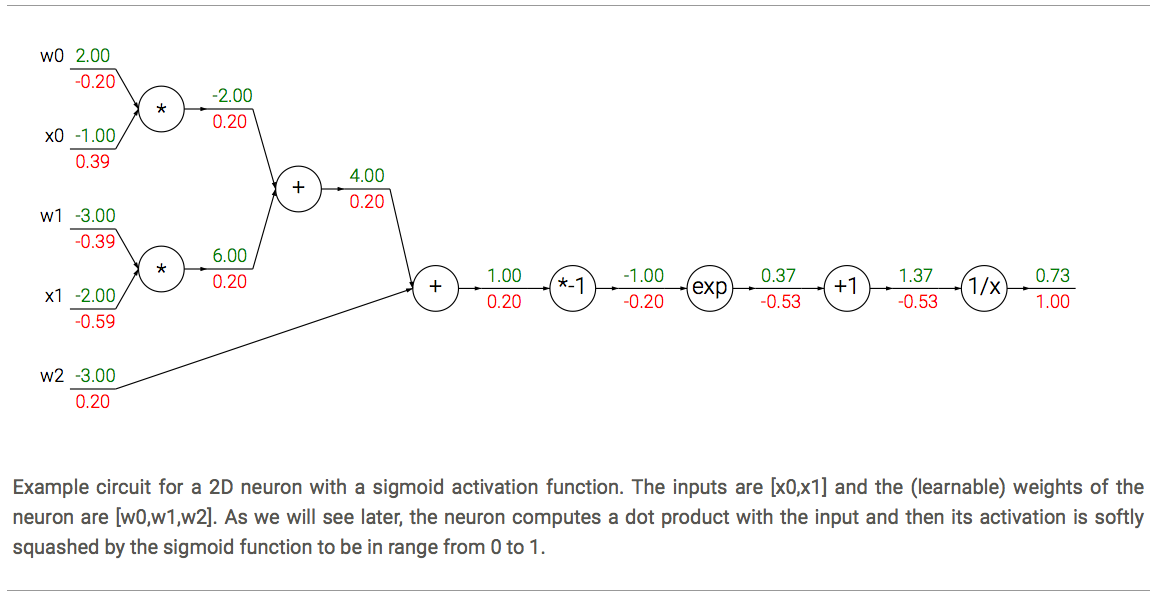
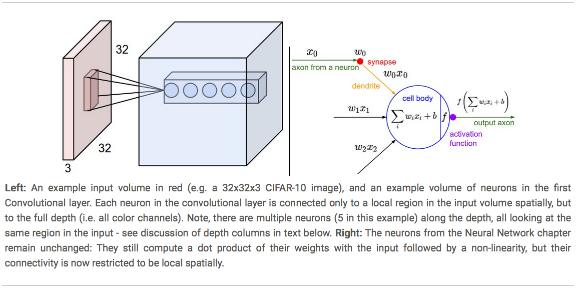
We model the neuron by two parts: linear combination \(\sum w_i x_i\) and activation function \(f\)

Choices for activation function

Fully-connected layer

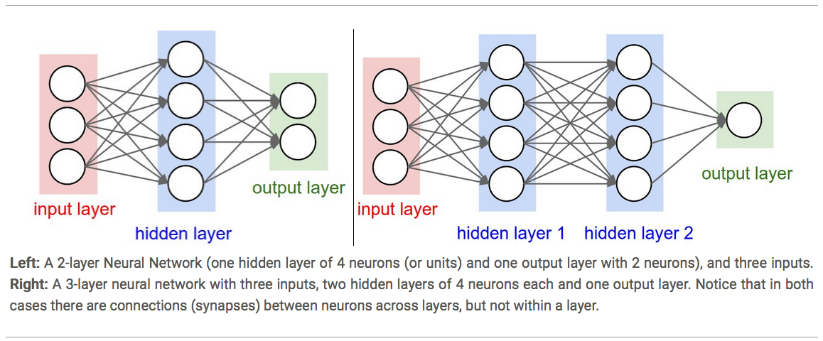
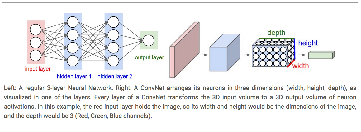
Total size of parameters (weights and biases) [input x #neuron]:
Left is (3 + 1) x 4 + (4 + 1) x 2 = 26.
Right is (3 + 1) x 4 + (4 + 1) x 4 + (4 + 1) x 1 = 41.

Example feed-forward computation

# forward-pass of a 3-layer neural network:
f = lambda x: np.where(x > 0, x, 0)  # ReLU activation
x = np.random.randn(3, 1)    # input vector (3x1)
h1 = f(np.dot(W1, x) + b1)   # 1st hidden layer (4x1)
h2 = f(np.dot(W2, h1) + b2)  # 2nd hidden layer (4x1)
out = np.dot(W3, h2) + b3    # output neuron (1x1)
      

The dim of Ws, bs: W1(4x3), b1(4x1), W2(4x4), b2(4x1), W3(4x1), b3(1x1)
Note that x can be (3xN) for batch input; no act. fun. in output layer.

Backward propagation

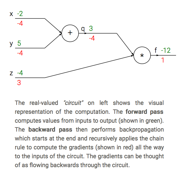
$$ \begin{aligned} f(x, y, z) = (x + y) z \\ q = x + y, \enspace f = qz \end{aligned} $$ $$ \begin{aligned} \Rightarrow \frac{\partial q}{\partial x} &= \frac{\partial q}{\partial y} = 1 \end{aligned} $$ $$ \begin{aligned} \Rightarrow \frac{\partial f}{\partial x} &= \frac{\partial f}{\partial q}\frac{\partial q}{\partial x} = z \cdot 1\\ \frac{\partial f}{\partial y} &= \frac{\partial f}{\partial q}\frac{\partial q}{\partial y} = z \cdot 1\\ \frac{\partial f}{\partial z} &= q \end{aligned} $$

# set some inputs
x = -2; y = 5; z = -4

# perform the forward pass
q = x + y  # q = 3
f = q * z  # f becomes -12

# perform the backward pass (back prop)
# in reverse order:
# first backprop through f = q * z
dfdz = q  # = 3
dfdq = z  # = -4
# now backprop through q = x + y
dfdx = 1.0 * dfdq  # = -4, dq/dx = 1
dfdy = 1.0 * dfdq  # = -4, dq/dy = 1
        

Backward propagation example

Think of a sigmoid function, \( f(w,x) = \frac{1}{1+e^{-(w_0x_0 + w_1x_1 + w_2)}} \).
First compute all the building blocks, $$ \begin{aligned} f(x) = \frac{1}{x} \quad &\rightarrow \quad \frac{df}{dx} = -1/x^2 \\ f_c(x) = c + x \quad &\rightarrow \quad \frac{df}{dx} = 1 \\ f(x) = e^x \quad &\rightarrow \quad \frac{df}{dx} = e^x = f(x) \\ f_a(x) = ax \quad &\rightarrow \quad \frac{df}{dx} = a \end{aligned} $$ Given initial w0, x0, w1, x1, w2 values (cont'd on next page)

Backward propagation example (cont'd)

Backprop in practice

Matrix-Matrix multiply gradient

# forward pass
W = np.random.randn(5, 10)
X = np.random.randn(10, 3)
D = W.dot(X)  # shape (5, 3)
# ... suppose we had the gradient on D from upper stage
dD = np.random.randn(*D.shape)  # same shape as D
dW = dD.dot(X.T)  # X.T = X's transpose matrix
dX = W.T.dot(dD)

Get our hands wet

Now we are able to make a 2-layer fully connected (FC) NN, which has the structure: input - FC layer - ReLU - FC layer - softmax - out class

It's in notebook 02.

But I'm afraid we are almost running out of time so probably just see the final result to get the whole picture.

Before learning: sanity checks tips/tricks

Back on parameter updates

v = mu * v - learning_rate * dx # integrate velocity
x += v # integrate position
          

Parameter update method comparison

Animations that may help your intuitions about the learning process dynamics. Left: Contours of a loss surface and time evolution of different optimization algorithms. Notice the "overshooting" behavior of momentum-based methods, which make the optimization look like a ball rolling down the hill. Right: A visualization of a saddle point in the optimization landscape, where the curvature along different dimension has different signs (one dimension curves up and another down). Notice that SGD has a very hard time breaking symmetry and gets stuck on the top. Conversely, algorithms such as RMSprop will see very low gradients in the saddle direction. Tue to the denominator term in the RMSprop update, this will increase the effective learning rate along this direction, helping RMSProp proceed.

Ref: CS231n Note: Neural Network 3 and Image credit: Alec Radford.

Convolutional Neural Network (CNN)

ConvNet introduces depth

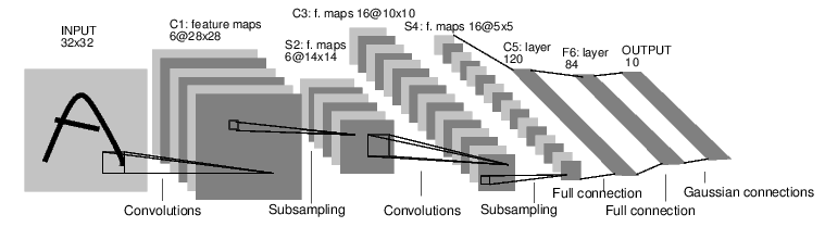
Input viewed as 32 width x 32 height x 3 channels (depth)
Output viewed as 1 x 1 x 10. Spatial information is preserved.

Receptive field: height and width of the spatially bounded input of all depths the neuron next stage takes from the former layer.

Convolutional layer - spatial arrangement

Receptive field vs output size example

Conv. layer - spatial arrangement (cont'd)

Conv. layer - parameter sharing

ImageNet 1st Conv layer filter visualization

Conv. layer - summary

Max Pooling Layer

Converting FC layer to CONV layers

An FC layer with \(K = 4096\) looking at Conv layer of [7x7x512] volumes, using filter size \(F = 7\) gives output volume [1x1x4096].

An FC layer looks at the previous layer with \(K = 1000\) and \(F=1\) gives output [1x1x1000].

That's all you need for a ConvNet :)

Layer Patterns

INPUT -> [[CONV -> RELU]*N -> POOL?]*M -> [FC -> RELU]*K -> FC

You should be able to read these CNNs

Get our hands wet

Notebook 03 works forward/backward implementation for all types of layer.

Notebook 04 creates a CONV-RELU-POOL-FC two-layer ConvNet.

What we've skipped

  • kNN classifier
  • SVM loss function
  • Gradient random local search
  • Other neuron activation functions
  • Overfitting/generalization tradeoff
  • Data preprocessing
  • L1 regularization
  • Dropout
  • Tips for tuing the learning process
  • Ratio of weights:updates
  • Other parameter update methods
  • Parameter search
  • We just scratched the surface of CNN, reread the whole part

If you like the content, go thank the original author (not me)

Thank You!

Fork me on Github